Note

This page is generated from the Jupyter notebook notebooks/08_wcc_phot_photometry.ipynb in the repository. You can download it and run it interactively.

wcc-phot: differential photometry of a WCC image series

Tutorial for wcc_phot, the photometry sibling of wcc_sim: it takes a series of simulated WCC frames of the same field, picks a target plus the N best reference stars (unsaturated, isolated, away from edges, closest in G to the target), re-centroids every star in every frame from its WCS-predicted position, and builds a differential (relative) light curve — with either aperture or PSF-fit fluxes.

Requirements: run with the py313 conda env kernel. The Gaia queries are cached in gaia_cache/, so after the first run this notebook works offline.

[1]:

import numpy as np
import matplotlib.pyplot as plt

import wcc_sim
import wcc_phot
from wcc_sim import simulate_field
from wcc_phot import run_photometry

plt.style.use('gks')
TEAL, RED, AMBER = '#00798c', '#d1495b', '#edae49'

print(f'wcc_sim {wcc_sim.__version__} | wcc_phot {wcc_phot.__version__}')

wcc_sim 0.1.0 | wcc_phot 0.1.0

1. Simulate a dithered series

Five 90 s exposures of the same Kepler-field pointing as notebook 01, on a 4096×4096 subarray (≈ 69″ × 69″), with sub-pixel pointing offsets between frames — the kind of drift the per-frame centroiding is there to follow. run_photometry accepts the SimulatedField objects directly (FITS paths work the same way).

[2]:

RA0, DEC0 = 291.0, 44.5      # deg, ICRS (Kepler field)
EXPTIME = 90.0               # s
PIX_DEG = 16.87e-3 / 3600.0  # one IMX455 pixel in degrees

dithers_px = [(0.0, 0.0), (0.4, -0.2), (-0.3, 0.3), (0.1, 0.5), (-0.5, -0.1)]
frames = []
for k, (dx, dy) in enumerate(dithers_px):
    frames.append(simulate_field(
        ra=RA0 + dx * PIX_DEG, dec=DEC0 + dy * PIX_DEG,
        sensorfilter='zwo:r', focus=0, exptime=EXPTIME, seed=42 + k,
        shape=(4096, 4096), cache_dir='gaia_cache',
    ))
print(f"{len(frames)} frames, {frames[0].params['n_sources']} Gaia sources each")

5 frames, 32 Gaia sources each

2. Pick a target and run aperture photometry

The IMX455 effective full well is only ~16 ke⁻ and the in-focus PSF puts ~8% of the flux in the peak pixel, so at 90 s any star brighter than G ≈ 18.2 saturates — we take the unsaturated star closest to G = 18.5. run_photometry asks for the 10 best references; in this sparse subfield only 7 survive the cuts, so it warns and continues. The default aperture radius is the 95% encircled-energy radius of the wcc-sim PSF model for this sensorfilter/focus/jitter, with the background annulus at 1.5–2.5 × r_ap.

[3]:

cat = frames[0].catalog
ok = np.asarray(cat['in_image']) & ~np.asarray(cat['saturated'])
gmag = np.asarray(cat['phot_g_mean_mag'], dtype=float)
target_id = int(np.asarray(cat['source_id'])[ok][np.argmin(np.abs(gmag[ok] - 18.5))])

res_ap = run_photometry(frames, target=target_id, method='aperture', n_ref=10)
p = res_ap.params
print(f"target {p['target_source_id']}: r_ap={p['r_ap']} px "
      f"(model EE={p['ee_fraction']:.3f}), annulus {p['r_in']}-{p['r_out']} px, "
      f"{p['n_ref']} refs")
res_ap.stars

/Users/gudmundurstefansson/Dropbox/mypylib/notebooks/GIT/wcc-sim/src/wcc_phot/select.py:74: UserWarning: only 7 of 10 requested reference stars usable
  warnings.warn(

target 2126245824998773888: r_ap=9.0 px (model EE=0.950), annulus 13.5-22.5 px, 7 refs

[3]:

Table length=8

star	role	source_id	ra	dec	gmag
int64	str6	int64	float64	float64	float64
0	target	2126245824998773888	290.9890463714144	44.49648012727523	18.62946128845215
1	ref	2126245790639056384	291.0028161167172	44.50461676375653	18.82853126525879
2	ref	2126245829297362176	290.98798994029636	44.50020075913573	19.419755935668945
3	ref	2126245756279295232	290.99211840952046	44.49629665426356	19.473852157592773
4	ref	2126245790639029504	291.0104300591018	44.49512296717736	19.576889038085938
5	ref	2126245794938018816	290.9966134142337	44.49911131045152	19.74286651611328
6	ref	2126245790639020032	291.0062397545951	44.49149253211353	20.31865119934082
7	ref	2126245898018198144	291.00928413138956	44.50399266810741	20.342300415039062

3. The field, with apertures

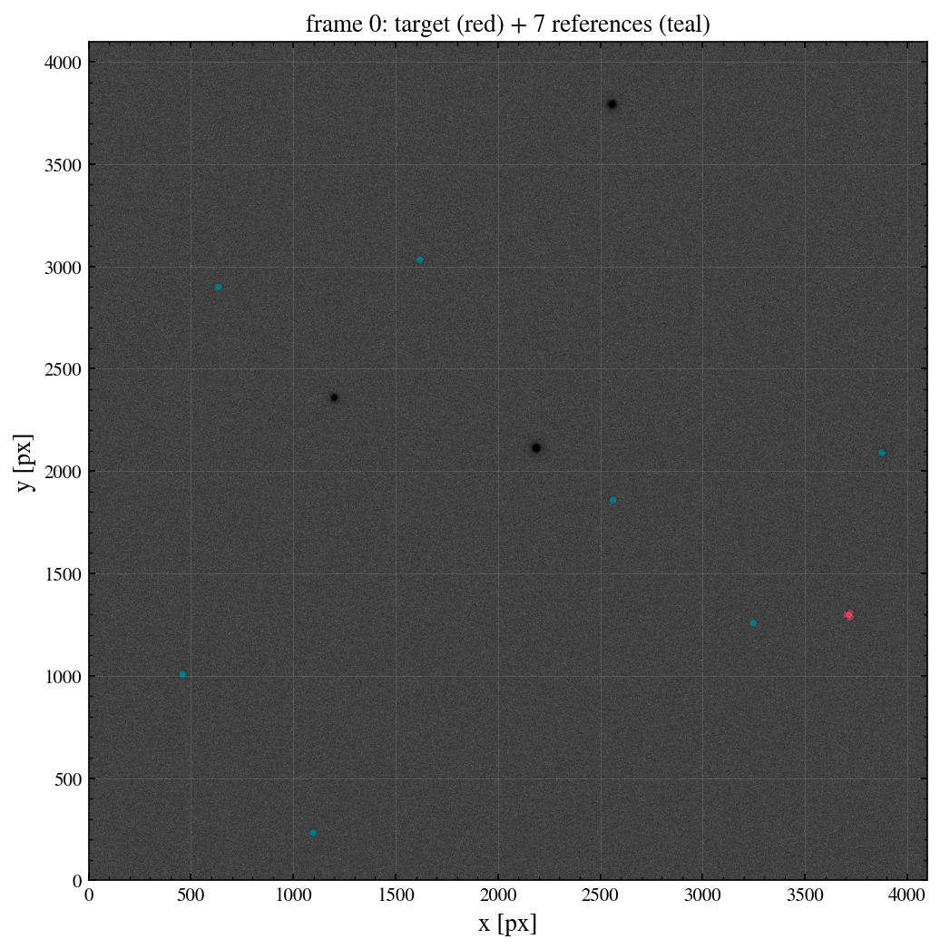
Target aperture + background annulus in red, reference apertures in teal, at the re-centroided positions measured on the first frame.

[4]:

from astropy.visualization import simple_norm
from matplotlib.patches import Circle

frame0 = frames[0]
m0 = res_ap.measurements[res_ap.measurements['frame'] == 0]

fig, ax = plt.subplots(figsize=(8.5, 8))
norm = simple_norm(frame0.image_e, 'asinh', percent=99.7)
ax.imshow(frame0.image_e, origin='lower', cmap='gray_r', norm=norm)
for row in m0:
    color = RED if row['role'] == 'target' else TEAL
    ax.add_patch(Circle((row['x'], row['y']), p['r_ap'], fill=False, color=color, lw=1.6))
    if row['role'] == 'target':
        for r in (p['r_in'], p['r_out']):
            ax.add_patch(Circle((row['x'], row['y']), r, fill=False,
                                color=RED, lw=0.9, ls='--', alpha=0.7))
ax.set_xlabel('x [px]'); ax.set_ylabel('y [px]')
ax.set_title(f"frame 0: target (red) + {p['n_ref']} references (teal)")
plt.show()

../_images/notebooks_08_wcc_phot_photometry_7_0.png

4. Relative light curve

The target flux is divided by the summed reference ensemble, normalized to its median. For a constant star the scatter should be consistent with the propagated photon + background + read-noise errors.

[5]:

lc = res_ap.lightcurve
rms = float(np.std(lc['rel_flux_norm']))
err = float(np.median(lc['rel_flux_norm_err']))

fig, ax = plt.subplots(figsize=(8, 4.5))
ax.errorbar(lc['time'], lc['rel_flux_norm'], yerr=lc['rel_flux_norm_err'],
            fmt='o', color=RED, ecolor=TEAL, capsize=3)
ax.axhline(1.0, color=TEAL, lw=0.8, ls=':')
ax.set_xlabel('frame'); ax.set_ylabel('normalized relative flux')
ax.set_title(f'rms {1e6*rms:.0f} ppm vs median error {1e6*err:.0f} ppm')
plt.show()

assert rms < 4 * err, 'light-curve scatter should match the propagated errors'
print(f'OK: rms {1e6*rms:.0f} ppm, consistent with {1e6*err:.0f} ppm errors')

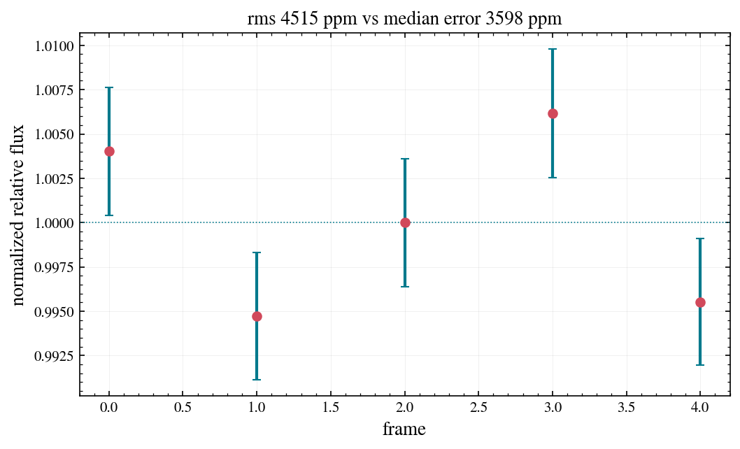
../_images/notebooks_08_wcc_phot_photometry_9_0.png

OK: rms 4515 ppm, consistent with 3598 ppm errors

5. Per-frame centroiding

Each star starts at its WCS-predicted position (x_init, y_init) in every frame — so the commanded dither is already taken out — and the center-of-mass refinement (x, y) absorbs what’s left. The predicted target position walks by up to half a pixel with the dither pattern; the centroid residuals stay well under a tenth of a pixel.

[6]:

mm = res_ap.measurements
tgt = mm[mm['role'] == 'target']

fig, (ax1, ax2) = plt.subplots(1, 2, figsize=(11, 4.3))
ax1.plot(tgt['frame'], tgt['x_init'] - tgt['x_init'][0], 'o-', color=TEAL, label='x')
ax1.plot(tgt['frame'], tgt['y_init'] - tgt['y_init'][0], 's-', color=AMBER, label='y')
ax1.set_xlabel('frame'); ax1.set_ylabel('WCS-predicted shift [px]')
ax1.set_title('dither seen by the WCS'); ax1.legend()

is_target = mm['role'] == 'target'
ax2.scatter(mm['x'][~is_target] - mm['x_init'][~is_target],
            mm['y'][~is_target] - mm['y_init'][~is_target],
            s=18, color=TEAL, label='refs')
ax2.scatter(mm['x'][is_target] - mm['x_init'][is_target],
            mm['y'][is_target] - mm['y_init'][is_target],
            s=30, color=RED, label='target')
ax2.axhline(0, color='0.7', lw=0.6); ax2.axvline(0, color='0.7', lw=0.6)
ax2.set_xlabel('x - x_init [px]'); ax2.set_ylabel('y - y_init [px]')
ax2.set_title('centroid residuals (all stars, all frames)'); ax2.legend()
plt.tight_layout(); plt.show()

max_resid = float(np.max(np.hypot(mm['x'] - mm['x_init'], mm['y'] - mm['y_init'])))
assert max_resid < 0.5, 'centroids should stay near the WCS prediction'
print(f'max centroid residual: {max_resid:.3f} px')

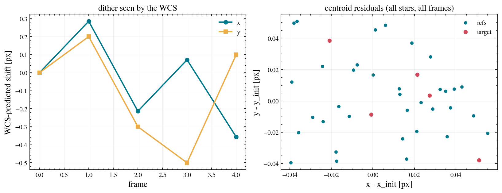
../_images/notebooks_08_wcc_phot_photometry_11_0.png

max centroid residual: 0.064 px

6. PSF photometry

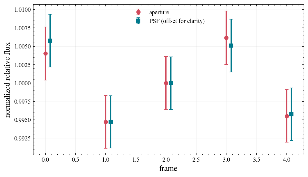
method='psf' fits every star with the same wcc-sim PSF model (rendered for this sensorfilter/focus/jitter and wrapped as a photutils ImagePSF), initialized from the centroid + aperture pass. PSF fluxes are total fluxes, so the aperture/PSF flux ratio of the target should sit near the model encircled-energy fraction at r_ap; the relative light curves should agree.

[7]:

res_psf = run_photometry(frames, target=target_id, method='psf', n_ref=10)

flux_ratio = float(np.median(
    res_ap.measurements['flux_e'][res_ap.measurements['role'] == 'target']
    / res_psf.measurements['flux_e'][res_psf.measurements['role'] == 'target']
))
print(f"aperture/PSF target flux ratio: {flux_ratio:.3f} "
      f"(model EE at r_ap: {p['ee_fraction']:.3f})")
assert abs(flux_ratio - p['ee_fraction']) < 0.05

lc_psf = res_psf.lightcurve
fig, ax = plt.subplots(figsize=(8, 4.5))
ax.errorbar(lc['time'], lc['rel_flux_norm'], yerr=lc['rel_flux_norm_err'],
            fmt='o', color=RED, capsize=3, label='aperture')
ax.errorbar(np.asarray(lc_psf['time']) + 0.08, lc_psf['rel_flux_norm'],
            yerr=lc_psf['rel_flux_norm_err'], fmt='s', color=TEAL, capsize=3,
            label='PSF (offset for clarity)')
ax.axhline(1.0, color='0.7', lw=0.8, ls=':')
ax.set_xlabel('frame'); ax.set_ylabel('normalized relative flux'); ax.legend()
plt.show()

/Users/gudmundurstefansson/Dropbox/mypylib/notebooks/GIT/wcc-sim/src/wcc_phot/select.py:74: UserWarning: only 7 of 10 requested reference stars usable
  warnings.warn(

aperture/PSF target flux ratio: 0.956 (model EE at r_ap: 0.950)

../_images/notebooks_08_wcc_phot_photometry_13_2.png

7. Watching it live

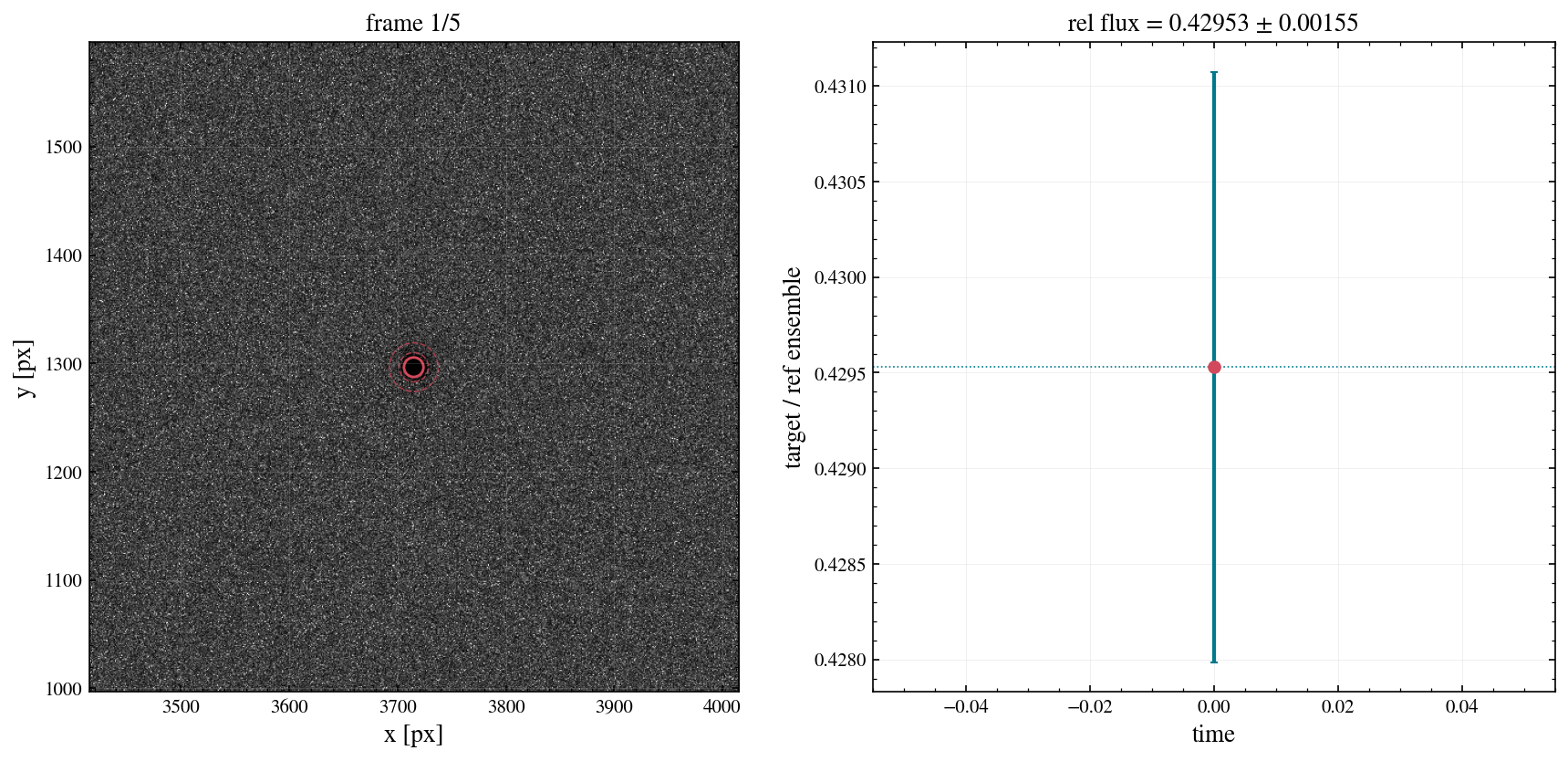
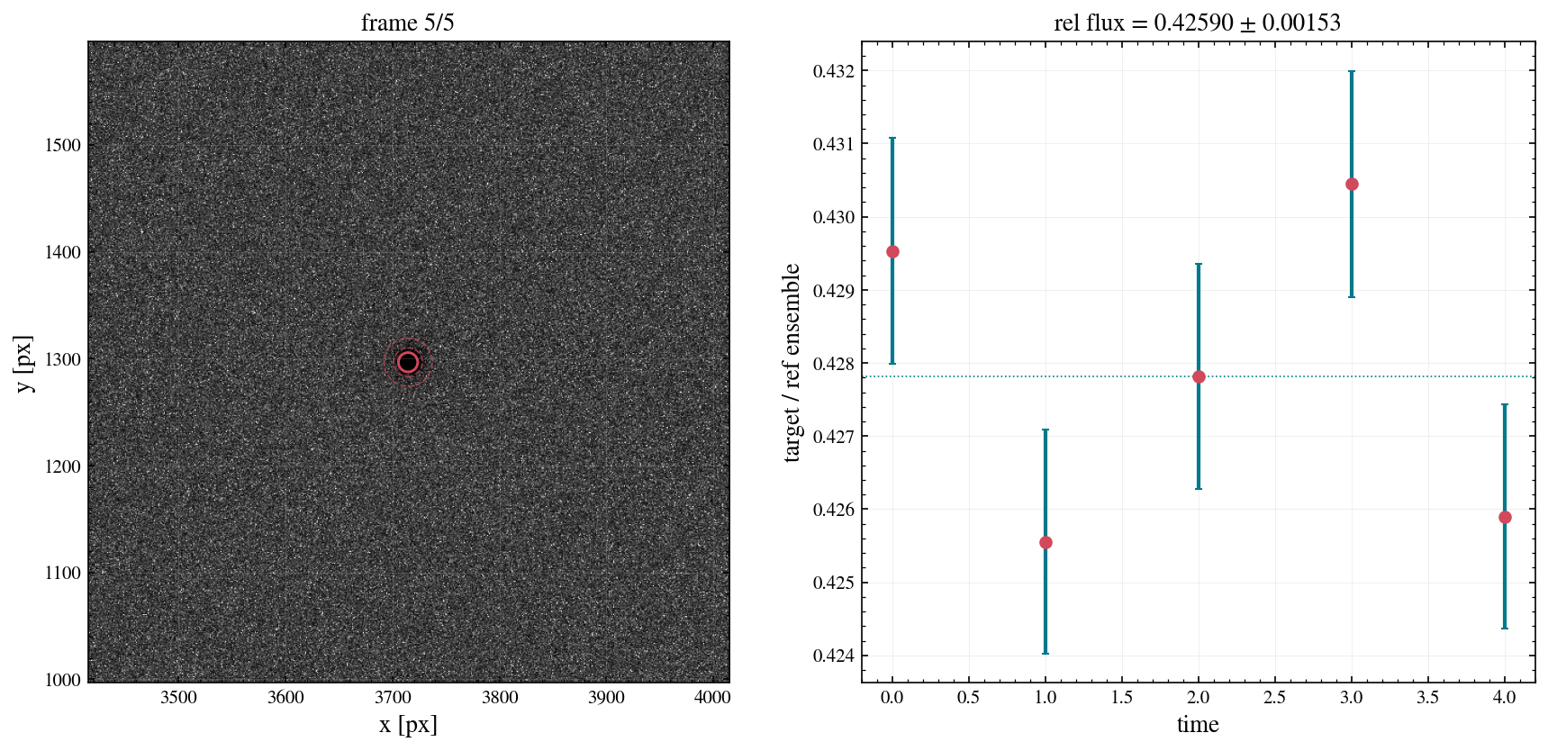
run_photometry(..., on_frame=...) calls any callable after each frame is measured with an event dict (image, centroided positions, geometry, fluxes, running relative flux) — that’s the hook for custom displays. wcc_phot.LiveViewer is the built-in matplotlib one: frame + apertures on the left, the growing light curve on the right, updated as each image is analyzed. From the shell it’s just:

wcc-phot series*.fits --source-id <id> --live -o phot.fits

(--live-zoom 250 crops the image panel around the target, --live-pause sets the update cadence). In a notebook the same viewer animates with an interactive backend (%matplotlib widget); with the inline backend we can still run it and show the final state:

[8]:

events = []
_ = run_photometry(frames[:2], target=target_id, n_ref=10, on_frame=events.append)
print('event keys:', sorted(events[0].keys()))
print('streamed rel_flux:', [round(e['rel_flux'], 4) for e in events])

/Users/gudmundurstefansson/Dropbox/mypylib/notebooks/GIT/wcc-sim/src/wcc_phot/select.py:74: UserWarning: only 7 of 10 requested reference stars usable
  warnings.warn(

event keys: ['flags', 'flux_e', 'flux_err_e', 'frame', 'geom', 'image_e', 'n_frames', 'rel_flux', 'rel_flux_err', 'roles', 'time', 'wcs', 'x', 'y']
streamed rel_flux: [0.4295, 0.4256]

[9]:

from wcc_phot import LiveViewer

viewer = LiveViewer(pause=0.01, zoom=300)
_ = run_photometry(frames, target=target_id, n_ref=10, on_frame=viewer)
viewer._fig

/Users/gudmundurstefansson/Dropbox/mypylib/notebooks/GIT/wcc-sim/src/wcc_phot/select.py:74: UserWarning: only 7 of 10 requested reference stars usable
  warnings.warn(

../_images/notebooks_08_wcc_phot_photometry_16_1.png

[9]:

../_images/notebooks_08_wcc_phot_photometry_16_2.png

Summary

run_photometry(frames, target, method='aperture'|'psf', n_ref=10) → target + best-N reference selection, per-frame WCS-seeded COM centroiding, model-PSF-driven aperture geometry (or ImagePSF fitting), ensemble relative light curve.
Results: .stars (selection), .measurements (per star per frame, with flags for centroid-fallback / saturation / edge), .lightcurve, .params; .write() saves a STARS/PHOT/LC FITS.
CLI: wcc-phot frames*.fits --source-id ... [--method psf] [--live] -o phot.fits (see scripts/example_photometry.sh).
Live displays hook in through on_frame — LiveViewer or anything you write.