Note
This page is generated from the Jupyter notebook
notebooks/01_getting_started.ipynb in the
repository. Download it and run it interactively to experiment.
1. Getting started
lazuli-exo simulates transmission spectroscopy with the Lazuli IFS. Give it a showcase planet, an atmosphere scenario and a number of transits, and it returns the model transmission spectrum binned to the instrument, the 1-sigma error bar per bin, and a spectral-template S/N.
import lazuli_exo needs numpy and nothing else. The atmosphere is a fast surrogate for POSEIDON (an interpolated opacity grid plus analytic scale-height, cloud and haze terms) and the noise comes from precomputed slicersim tables.
What the numbers mean. The instrument half (photon and read noise through the real throughput, readout and line-spread function) is quantitative. The atmosphere half is a 1D isothermal, equilibrium-chemistry surrogate with statistical noise only: no P-T profile, no systematics floor. Use the outputs for rankings and trade studies. Do not quote the template S/N as a detection significance. Known approximations lists what the model leaves out.
[1]:
import numpy as np
import matplotlib.pyplot as plt

try:
    plt.style.use("gks")
except OSError:
    pass

import lazuli_exo

print("lazuli_exo", lazuli_exo.__version__ if hasattr(lazuli_exo, "__version__") else "(dev)")
lazuli_exo (dev)
What is available
Fourteen showcase targets, each with the same five scenarios. list_planets() reads the table index; list_scenarios() returns the preset names.
[2]:
planets = lazuli_exo.list_planets()
print(f"{len(planets)} showcase targets\n")
for p in planets:
    print(f"  {p:14s} {lazuli_exo.list_scenarios(p)}")
14 showcase targets

  GJ 1214 b      ['clear', 'cloudy', 'flat', 'hazy', 'high_metallicity']
  GJ 3470 b      ['clear', 'cloudy', 'flat', 'hazy', 'high_metallicity']
  HAT-P-11 b     ['clear', 'cloudy', 'flat', 'hazy', 'high_metallicity']
  HD 189733 b    ['clear', 'cloudy', 'flat', 'hazy', 'high_metallicity']
  HD 209458 b    ['clear', 'cloudy', 'flat', 'hazy', 'high_metallicity']
  K2-18 b        ['clear', 'cloudy', 'flat', 'hazy', 'high_metallicity']
  LHS 1140 b     ['clear', 'cloudy', 'flat', 'hazy', 'high_metallicity']
  TOI-270 d      ['clear', 'cloudy', 'flat', 'hazy', 'high_metallicity']
  TRAPPIST-1 e   ['clear', 'cloudy', 'flat', 'hazy', 'high_metallicity']
  WASP-107 b     ['clear', 'cloudy', 'flat', 'hazy', 'high_metallicity']
  WASP-12 b      ['clear', 'cloudy', 'flat', 'hazy', 'high_metallicity']
  WASP-121 b     ['clear', 'cloudy', 'flat', 'hazy', 'high_metallicity']
  WASP-39 b      ['clear', 'cloudy', 'flat', 'hazy', 'high_metallicity']
  WASP-96 b      ['clear', 'cloudy', 'flat', 'hazy', 'high_metallicity']
A single observation
observe() takes a planet name, a scenario, the number of transits to co-add and the resolving power R to bin the spectrum to.
[3]:
import dataclasses

obs = lazuli_exo.observe("WASP-39 b", scenario="clear",
                         n_transits=1, R=100)
print(type(obs).__name__, "fields:",
      ", ".join(f.name for f in dataclasses.fields(obs)))
SimulatedSpectrum fields: planet, scenario, n_transits, R, wavelength, depth, depth_err, model_wavelength, model_depth, flat_depth, meta
Anatomy of a SimulatedSpectrum
The result is a plain dataclass. You will use wavelength, depth and depth_err most; model_wavelength and model_depth keep the native-resolution model for overplotting.
[4]:
for name in ["wavelength", "depth", "depth_err",
             "model_wavelength", "model_depth"]:
    arr = getattr(obs, name)
    print(f"{name:18s} shape={str(arr.shape):8s} "
          f"[{arr.min():.6g}, {arr.max():.6g}]")

print()
print(f"{'flat_depth':18s} {obs.flat_depth:.6g}   "
      "# geometric (Rp/Rs)^2 from the registry radii")
print(f"{'R':18s} {obs.R}")
print(f"{'n_transits':18s} {obs.n_transits}")
wavelength         shape=(145,)   [0.401907, 1.68358]
depth              shape=(145,)   [0.0202449, 0.0231421]
depth_err          shape=(145,)   [7.48483e-05, 0.000326857]
model_wavelength   shape=(14430,) [0.399791, 1.69245]
model_depth        shape=(14430,) [0.0199945, 0.0279577]

flat_depth         0.0212285   # geometric (Rp/Rs)^2 from the registry radii
R                  100
n_transits         1
The bins are constant resolving power (snapped to whole detector pixels), so the bin width grows with wavelength. depth is the noiseless model seen through the instrument and averaged into those bins; depth_err is the per-bin 1-sigma uncertainty.
[5]:
dlam = np.diff(obs.wavelength)
print(f"{obs.wavelength.size} bins from {obs.wavelength[0]:.3f} "
      f"to {obs.wavelength[-1]:.3f} um")
print(f"bin width: {dlam[0] * 1e3:.2f} nm at the blue end, "
      f"{dlam[-1] * 1e3:.2f} nm at the red end")
print(f"R implied at mid-band: "
      f"{obs.wavelength[len(dlam) // 2] / dlam[len(dlam) // 2]:.0f}")

print(f"\ndepth_err: median {np.median(obs.depth_err) * 1e6:.0f} ppm, "
      f"best {obs.depth_err.min() * 1e6:.0f} ppm, "
      f"worst {obs.depth_err.max() * 1e6:.0f} ppm")
145 bins from 0.402 to 1.684 um
bin width: 4.12 nm at the blue end, 15.73 nm at the red end
R implied at mid-band: 100

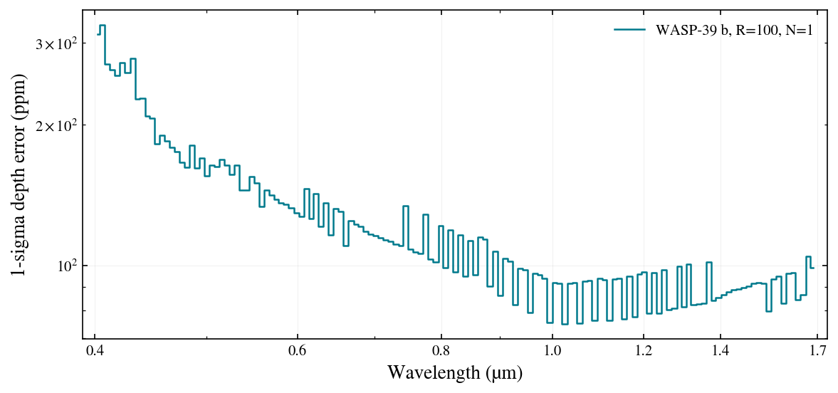
depth_err: median 107 ppm, best 75 ppm, worst 327 ppm
Plotting
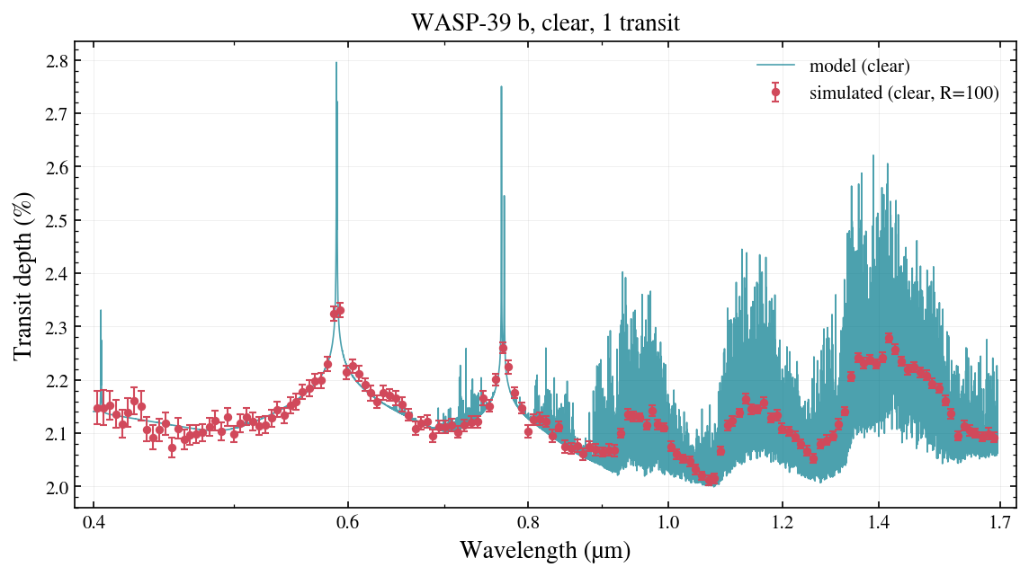
obs.plot() draws the native-resolution model with one simulated noisy realization at the binned resolution. It needs the [plot] extra (matplotlib). Every plot method takes an optional ax and returns the Axes, so you can pass your own subplot or overlay several calls; notebook 2 does that.
[6]:
obs.plot(seed=0)
plt.show()
obs.plot_noise() shows where the instrument is precise: the per-bin 1-sigma error against wavelength, with n_transits already included.
[7]:
obs.plot_noise()
plt.show()
Noise realizations
depth and depth_err are deterministic. The noise is drawn on demand by simulate_points(seed), and a seed makes a realization reproducible, which is how the web demo and these notebooks stay stable across runs.
[8]:
a = obs.simulate_points(seed=0)
b = obs.simulate_points(seed=0)
c = obs.simulate_points(seed=1)

assert np.array_equal(a, b), "same seed must give the same realization"
assert not np.array_equal(a, c), "different seeds must differ"

resid = (a - obs.depth) / obs.depth_err
print(f"same seed reproduces:      {np.array_equal(a, b)}")
print(f"different seed differs:    {not np.array_equal(a, c)}")
print(f"\nresiduals in sigma units: mean {resid.mean():+.3f}, "
      f"std {resid.std():.3f}  (expect ~0 and ~1)")
same seed reproduces:      True
different seed differs:    True

residuals in sigma units: mean +0.080, std 0.954  (expect ~0 and ~1)
Detection diagnostics
obs.detect() returns a matched-template amplitude S/N of the noiseless model against the best-fit flat line, under a diagonal covariance.
template_snr_diagonal is a comparison statistic, not a calibrated detection significance: there is no likelihood ratio, no nuisance model, no covariance and no false-positive calibration. The per-band values are the same statistic restricted to fixed wavelength masks. They mix every species in the mask with the haze, cloud and continuum structure, and the masks overlap, so they are not molecule detections either.
[9]:
result = obs.detect()

print(f"template_snr_diagonal: {result['template_snr_diagonal']:.1f}\n")
print("band_snr (band-restricted template norms, NOT detections):")
for mol, snr in sorted(result["band_snr"].items(),
                       key=lambda kv: -kv[1]):
    print(f"  {mol:5s} {snr:7.1f}")
template_snr_diagonal: 68.6

band_snr (band-restricted template norms, NOT detections):
  H2O      46.6
  CO2      26.0
  Na       22.7
  CH4      18.8
  K        15.2
The band masks live in lazuli_exo.detect.BAND_MASKS. H2O and CH4 both cover 1.10 to 1.20 µm, which is one reason these are not per-molecule detections.
[10]:
from lazuli_exo.detect import BAND_MASKS

for mol, spans in BAND_MASKS.items():
    pretty = ", ".join(f"{lo:.3f}-{hi:.3f}" for lo, hi in spans)
    print(f"  {mol:5s} {pretty} um")
  Na    0.575-0.605 um
  K     0.755-0.785 um
  H2O   0.900-1.000, 1.100-1.200, 1.300-1.550 um
  CH4   0.860-0.910, 1.100-1.200, 1.600-1.700 um
  CO2   1.420-1.460, 1.560-1.620 um
Where the numbers came from
Every observation carries its provenance in obs.meta: the parameters the model was evaluated at (params), what the atmosphere model derived from them (atmosphere), the slicersim settings behind the error bars (noise) and how the model was put through the spectrograph (instrument_response). This is the first place to look when a number surprises you.
[11]:
SHOW = {
    "params": ["T_eq_K", "R_p_RJ", "M_p_MJ", "R_s_RSun", "log_met", "c_to_o",
               "mu", "log_P_cloud_bar", "log_a_haze"],
    "atmosphere": ["g_ms2", "H_m", "H_over_Rp", "mu_used", "mu_source",
                   "T_chem_K", "T_clamped", "feature_amplitude_ppm"],
    "noise": ["instrument", "nmd_used", "t14_s", "t_obs_s", "mag_input", "mag_ab",
              "fully_desaturated", "nsaturated_detpx", "slicersim_version",
              "git_commit"],
    "instrument_response": None,          # all keys
}
for section, keys in SHOW.items():
    d = obs.meta[section]
    print(f"meta[{section!r}]:")
    for k in keys or d:
        v = d[k]
        print(f"  {k:22s} {v:.6g}" if isinstance(v, float) else f"  {k:22s} {v}")
    print()
meta['params']:
  T_eq_K                 1166
  R_p_RJ                 1.33134
  M_p_MJ                 0.281
  R_s_RSun               0.939
  log_met                0
  c_to_o                 0.55
  mu                     None
  log_P_cloud_bar        None
  log_a_haze             None

meta['atmosphere']:
  g_ms2                  3.92911
  H_m                    1.05466e+06
  H_over_Rp              0.0110807
  mu_used                2.32131
  mu_source              chemistry
  T_chem_K               1166
  T_clamped              False
  feature_amplitude_ppm  7963.21

meta['noise']:
  instrument             lazuli_cbe
  nmd_used               [2, 8, 0]
  t14_s                  10091.5
  t_obs_s                48.11
  mag_input              10.663
  mag_ab                 11.5623
  fully_desaturated      True
  nsaturated_detpx       0
  slicersim_version      1.3.4
  git_commit             7d0f71b1f0a36437226d6d26346c74f6baa8dc1f

meta['instrument_response']:
  lsf_sigma_px           1.15
  resolution_px          2.3
  R_instr_min            100.596
  R_instr_max            368.731
  photon_weighting       star table R=10000
  edges_snapped          True
Summary
lazuli_exo.observe(planet, scenario, n_transits, R)returns aSimulatedSpectrum..depthand.depth_errare the noiseless model and its 1-sigma errors;.simulate_points(seed)draws a reproducible noisy realization..plot(),.plot_noise()and (notebook 4).light_curves().plot()all takeax=and return the Axes..detect()gives a template S/N: a comparison statistic, not a significance..metarecords the parameters, the derived atmosphere quantities and the noise settings that produced the numbers.
Next: scenarios, what the five atmosphere scenarios mean and how they differ.