Note

This page is generated from the Jupyter notebook notebooks/04_light_curves.ipynb in the repository. Download it and run it interactively to experiment.

4. Transit light curves

obs.light_curves() turns a simulated spectrum into the time domain: one white-light curve, or several split by wavelength band so you can watch the transit depth change with colour.

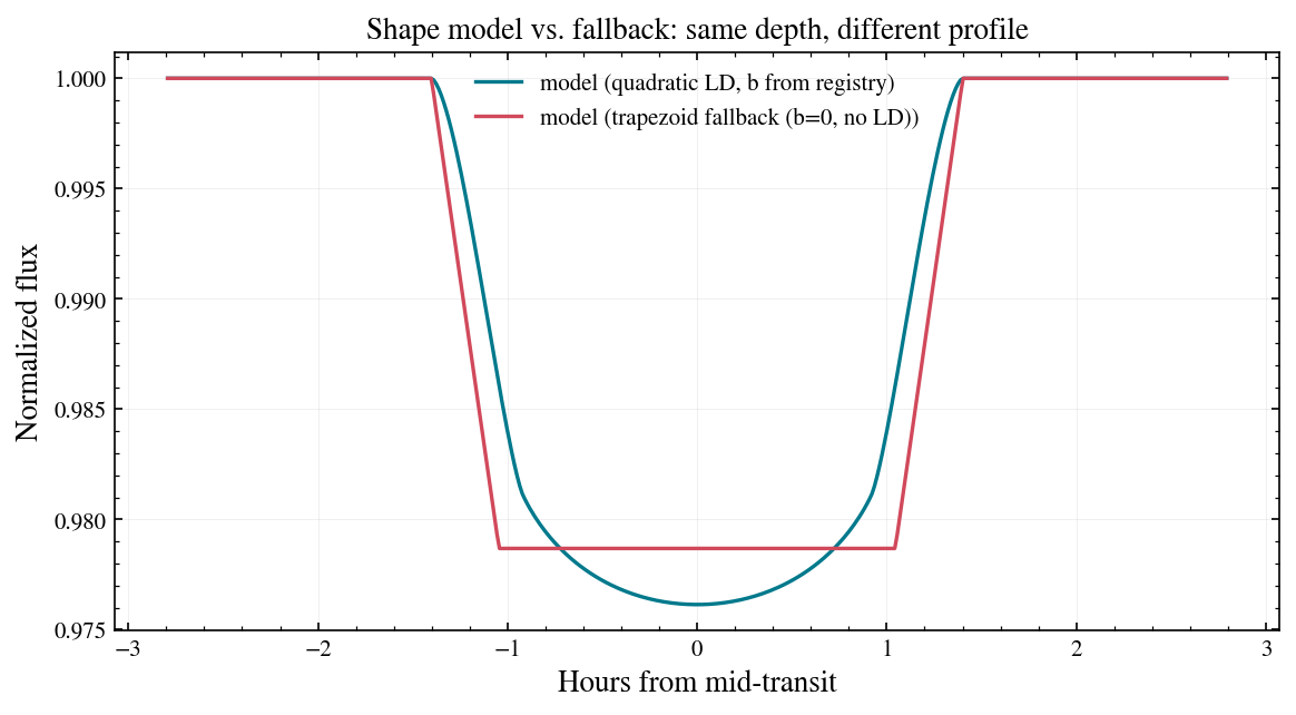
The shape is a quadratically limb-darkened transit computed by numpy-only numerical disk integration. The geometry comes from the frozen NASA Exoplanet Archive registry, with z(t) the exact sky-projected separation of the Keplerian orbit, and the limb-darkening coefficients from per-planet exotic-ld tables. Planets with no registry entry or no LD table fall back to a b = 0 trapezoid, and meta["shape"] records which model was used.

import numpy as np
import matplotlib.pyplot as plt

try:
    plt.style.use("gks")
except OSError:
    pass

import lazuli_exo

print("lazuli_exo", lazuli_exo.__version__ if hasattr(lazuli_exo, "__version__") else "(dev)")

lazuli_exo (dev)

The white-light curve

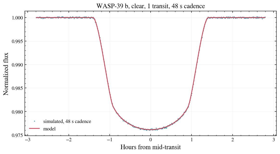
With n_groups=1 every spectral bin is combined into a single light curve. The observation window is ±t14 around mid-transit (the equal out-of-transit baseline the noise tables assume), sampled at the instrument’s native integration time. lc.plot() draws the noisy realization over the model.

PLANET = "WASP-39 b"

obs = lazuli_exo.observe(PLANET, scenario="clear", n_transits=1, R=100)
lc = obs.light_curves(n_groups=1, seed=0)

print(f"labels:      {lc.labels}")
print(f"time_hr:     {lc.time_hr.size} samples, "
      f"{lc.time_hr[0]:+.2f} to {lc.time_hr[-1]:+.2f} h")
print(f"cadence:     {lc.cadence_s:.2f} s")
print(f"t14:         {lc.t14_s:.1f} s  ({lc.t14_s / 3600:.2f} h)")
print(f"depth:       {lc.depth[0] * 100:.4f} %")
print(f"sigma/point: {lc.sigma_point[0] * 1e6:.1f} ppm")
print(f"\nmeta: {lc.meta}")

labels:      ['white light']
time_hr:     419 samples, -2.79 to +2.79 h
cadence:     48.11 s
t14:         10091.5 s  (2.80 h)
depth:       2.1316 %
sigma/point: 90.9 ppm

meta: {'planet': 'WASP-39 b', 'scenario': 'clear', 'n_transits': 1, 'shape': 'quadratic-ld', 'b': 0.532570994641176, 'a_over_rs': 11.39, 't14_geom_s': 9960.196814117857, 'time_stretch': 0.9869867784157249}

lc.plot()
plt.show()

Wavelength-banded light curves

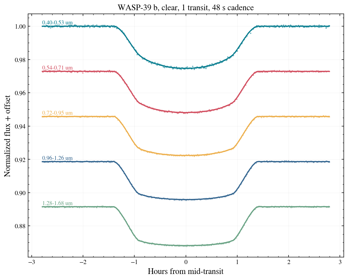
n_groups > 1 splits the spectrum into contiguous bands of equal bin count. The geometry is shared, and each band gets its own depth and its own limb darkening, so the curves are not scaled copies of one another. lcb.plot() stacks them with an offset; pass offset= to change the spacing.

lcb = obs.light_curves(n_groups=5, seed=0)

print(f"{'band':18s}{'depth (%)':>11s}{'u1':>8s}{'u2':>8s}"
      f"{'sigma/pt (ppm)':>16s}")
for i, lab in enumerate(lcb.labels):
    print(f"{lab:18s}{lcb.depth[i] * 100:11.4f}"
          f"{lcb.u1[i]:8.3f}{lcb.u2[i]:8.3f}"
          f"{lcb.sigma_point[i] * 1e6:16.1f}")

band                depth (%)      u1      u2  sigma/pt (ppm)
0.40-0.53 um           2.1176   0.782   0.056           365.7
0.54-0.71 um           2.1639   0.536   0.162           246.8
0.72-0.95 um           2.1162   0.385   0.179           199.0
0.96-1.26 um           2.0950   0.292   0.195           164.4
1.28-1.68 um           2.1696   0.176   0.272           169.6

lcb.plot()
plt.show()

Validating transit_flux

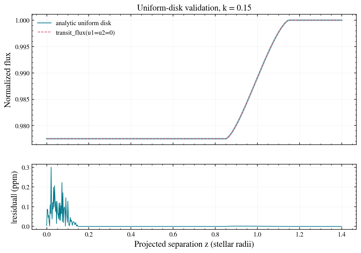
The occultation model is lazuli_exo.lightcurve.transit_flux(z, k, u1, u2): normalized flux for an opaque disk of radius ratio k at projected separations z in stellar radii. With u1 = u2 = 0 it must reduce to the analytic uniform-disk overlap, a closed-form expression, so the check is worth running rather than assuming.

from lazuli_exo.lightcurve import transit_flux


def uniform_disk_flux(z, k):
    """Analytic uniform-source occultation (Mandel & Agol 2002, lambda_e)."""
    z = np.abs(np.asarray(z, float))
    out = np.ones_like(z)

    full = z <= 1.0 - k                      # planet fully on the disk
    out[full] = 1.0 - k ** 2

    part = (np.abs(1.0 - k) < z) & (z <= 1.0 + k)   # partial overlap
    zp = z[part]
    k0 = np.arccos((k ** 2 + zp ** 2 - 1.0) / (2.0 * k * zp))
    k1 = np.arccos((1.0 - k ** 2 + zp ** 2) / (2.0 * zp))
    area = (k ** 2 * k0 + k1
            - np.sqrt(4.0 * zp ** 2 - (1.0 + zp ** 2 - k ** 2) ** 2) / 2.0)
    out[part] = 1.0 - area / np.pi
    return out


z = np.linspace(0.0, 1.4, 601)
k = 0.15

numeric = transit_flux(z, k, 0.0, 0.0)
analytic = uniform_disk_flux(z, k)
err = np.abs(numeric - analytic)

print(f"k = {k}, {z.size} separations")
print(f"max |numeric - analytic|: {err.max():.3e}")
print(f"in ppm of the depth:      {err.max() / k ** 2 * 1e6:.2f} ppm")

assert err.max() < 1e-5, "uniform-disk limit must be recovered"
print("\nOK: the uniform-disk limit is recovered.")

k = 0.15, 601 separations
max |numeric - analytic|: 3.005e-07
in ppm of the depth:      13.35 ppm

OK: the uniform-disk limit is recovered.

fig, (ax1, ax2) = plt.subplots(2, 1, figsize=(9, 6), sharex=True,
                               gridspec_kw={"height_ratios": [2, 1]})

ax1.plot(z, analytic, lw=2.4, alpha=0.5, label="analytic uniform disk")
ax1.plot(z, numeric, lw=1.0, ls="--", label="transit_flux(u1=u2=0)")
ax1.set_ylabel("Normalized flux")
ax1.legend(frameon=False)
ax1.set_title(f"Uniform-disk validation, k = {k}")

ax2.plot(z, err * 1e6, lw=1.0)
ax2.set_xlabel("Projected separation z (stellar radii)")
ax2.set_ylabel("|residual| (ppm)")
plt.show()

Limb darkening

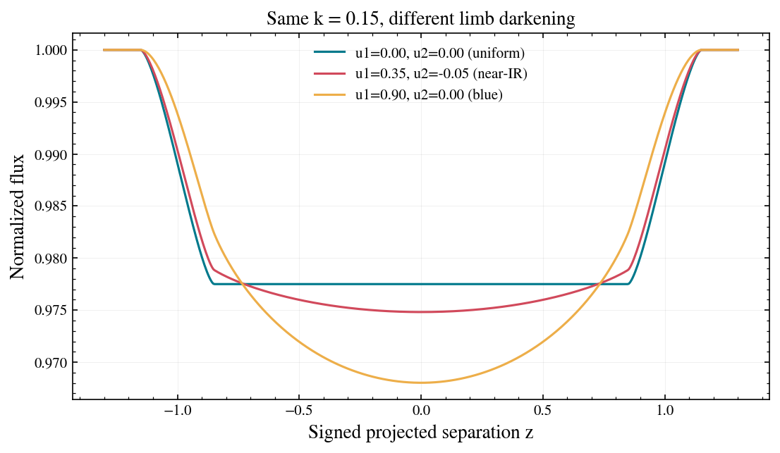
The coefficients come from per-planet tables built with exotic-ld on a PHOENIX grid, refit under the Kipping (2013) constraints so the intensity profile stays physical. They vary strongly across the band, with much stronger limb darkening in the blue than in the near-IR, which is why the banded curves above change shape as well as depth.

from lazuli_exo import tables

tdir = tables.resolve_tables_dir(None)
wl_ld, u1_ld, u2_ld, ld_meta = tables.load_ld(tdir, PLANET)

fig, ax = plt.subplots(figsize=(8.5, 4.2))
ax.plot(wl_ld, u1_ld, "o-", ms=3, label="u1")
ax.plot(wl_ld, u2_ld, "o-", ms=3, label="u2")
ax.set_xlabel("Wavelength (µm)")
ax.set_ylabel("Quadratic LD coefficient")
ax.set_title(f"{PLANET}: limb darkening ({ld_meta['ld_grid']}, "
             f"{ld_meta['law']})")
ax.legend(frameon=False)
plt.show()

print(f"grid point used: Teff={ld_meta['Teff_used']}, "
      f"logg={ld_meta['logg_used']}, M_H={ld_meta['M_H_used']}")
print(f"inputs clamped to grid: {ld_meta['inputs_clamped']}")
print(f"{wl_ld.size} wavelength chunks over "
      f"{ld_meta['wl_range_um']} um")

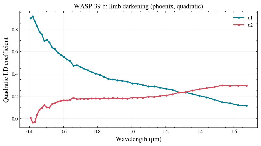
grid point used: Teff=5485.0, logg=4.453, M_H=0.01
inputs clamped to grid: []
48 wavelength chunks over [0.4, 1.7] um

The effect on the curve shape is easiest to see by holding the depth fixed and sweeping the coefficients.

fig, ax = plt.subplots(figsize=(8.5, 4.5))

zz = np.linspace(-1.3, 1.3, 501)
for u1, u2, lab in [(0.0, 0.0, "u1=0.00, u2=0.00 (uniform)"),
                    (0.35, -0.05, "u1=0.35, u2=-0.05 (near-IR)"),
                    (0.90, 0.00, "u1=0.90, u2=0.00 (blue)")]:
    ax.plot(zz, transit_flux(np.abs(zz), 0.15, u1, u2), lw=1.5, label=lab)

ax.set_xlabel("Signed projected separation z")
ax.set_ylabel("Normalized flux")
ax.set_title("Same k = 0.15, different limb darkening")
ax.legend(frameon=False)
plt.show()

Geometry from the registry

The impact parameter and the orbit come from the frozen registry: b from a/R* and cos i with an eccentricity factor, and z(t) from Kepler’s equation (lazuli_exo.orbit.projected_separation) with mid-transit at inferior conjunction, so z(0) = b exactly.

The registry t14 is the measured archive duration and sets the noise and the window. The geometric duration from (P, a/R*, k, i, e, ω) can differ, so the orbit clock is stretched by their ratio and the model’s first-to-fourth-contact duration equals t14. Both numbers are in lc.meta.

from lazuli_exo.targets import get_target

t = get_target(PLANET)
for key in ["period_d", "a_over_rs", "inc_deg", "ecc", "w_deg", "t14_s",
            "depth", "provenance"]:
    print(f"  {key:12s} {t[key]}")

print(f"\nderived by light_curves(): shape={lc.meta['shape']}, "
      f"b={lc.meta['b']:.3f}, a/Rs={lc.meta['a_over_rs']}, "
      f"t14_geom={lc.meta['t14_geom_s']:.0f} s, "
      f"time_stretch={lc.meta['time_stretch']:.4f}")

  period_d     4.0552941
  a_over_rs    11.39
  inc_deg      87.32
  ecc          0.0
  w_deg        90.0
  t14_s        10091.52
  depth        0.02122849
  provenance   NEA PSCompPars

derived by light_curves(): shape=quadratic-ld, b=0.533, a/Rs=11.39, t14_geom=9960 s, time_stretch=0.9870

The trapezoid fallback

If a planet is not in the registry, or has no LD table, the shape falls back to a b = 0 trapezoid with no limb darkening. Relabelling an observation is enough to trigger it, and meta["shape"] tells you it happened. plot(ax=ax, show_points=False, label=...) overlays the two models.

import dataclasses

synthetic = dataclasses.replace(obs, planet="Synthetic b")
lc_fallback = synthetic.light_curves(n_groups=1, seed=0)

print(f"registry planet: shape={lc.meta['shape']!r}, "
      f"u1={lc.u1[0]:.3f}")
print(f"synthetic name:  shape={lc_fallback.meta['shape']!r}, "
      f"u1={lc_fallback.u1}")

assert lc.meta["shape"] == "quadratic-ld"
assert lc_fallback.meta["shape"] == "trapezoid"
assert lc_fallback.u1 is None

registry planet: shape='quadratic-ld', u1=0.434
synthetic name:  shape='trapezoid', u1=None

fig, ax = plt.subplots(figsize=(9, 4.5))
lc.plot(ax=ax, show_points=False, label="quadratic LD, b from registry")
lc_fallback.plot(ax=ax, show_points=False, label="trapezoid fallback (b=0, no LD)")
ax.set_title("Shape model vs. fallback: same depth, different profile")
plt.show()

Per-point noise

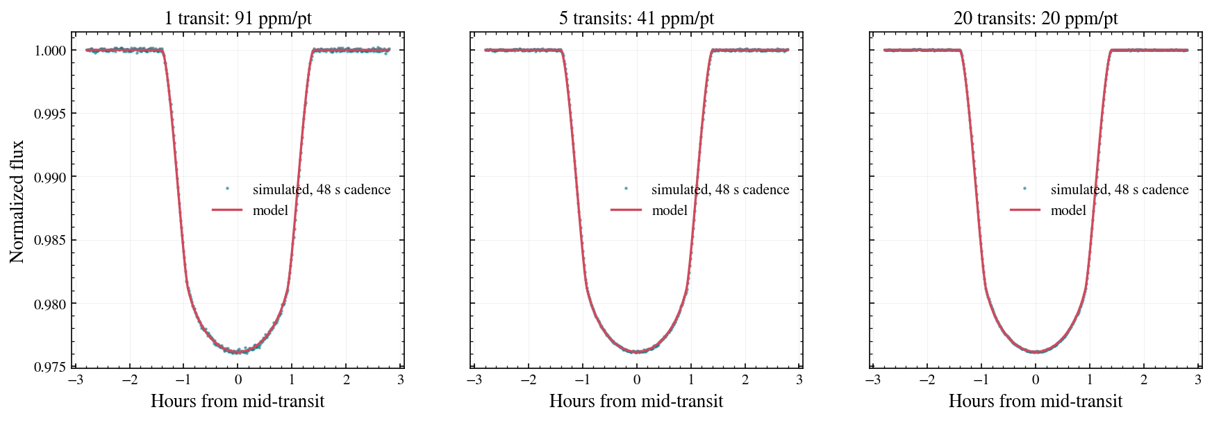
The scatter per sample is derived from the band’s depth precision rather than computed independently: σpt = σband √(t14/2c) for cadence c. This keeps the light curves consistent with the same equal out-of-transit baseline assumption the spectra use.

# reconstruct the band-combined depth precision from the public arrays:
# contiguous equal-count groups, combined in inverse variance
groups = np.array_split(np.arange(obs.depth.size), 5)
w = 1.0 / obs.depth_err ** 2
sigma_band = np.array([1.0 / np.sqrt(w[g].sum()) for g in groups])

expected = sigma_band * np.sqrt(lcb.t14_s / (2.0 * lcb.cadence_s))

print(f"{'band':18s}{'sigma_band (ppm)':>18s}{'sigma_pt (ppm)':>16s}"
      f"{'expected':>12s}")
for i, lab in enumerate(lcb.labels):
    print(f"{lab:18s}{sigma_band[i] * 1e6:18.1f}"
          f"{lcb.sigma_point[i] * 1e6:16.1f}{expected[i] * 1e6:12.1f}")

assert np.allclose(lcb.sigma_point, expected)
print("\nOK: sigma_pt = sigma_band * sqrt(t14 / 2c).")

band                sigma_band (ppm)  sigma_pt (ppm)    expected
0.40-0.53 um                    35.7           365.7       365.7
0.54-0.71 um                    24.1           246.8       246.8
0.72-0.95 um                    19.4           199.0       199.0
0.96-1.26 um                    16.1           164.4       164.4
1.28-1.68 um                    16.6           169.6       169.6

OK: sigma_pt = sigma_band * sqrt(t14 / 2c).

Co-adding transits sharpens the light curves the same way it sharpens the spectra: the per-point scatter drops as 1/√N while the model is unchanged.

fig, axes = plt.subplots(1, 3, figsize=(14, 4.2), sharey=True)

for ax, n in zip(axes, [1, 5, 20]):
    o = lazuli_exo.observe(PLANET, scenario="clear", n_transits=n, R=100)
    curve = o.light_curves(n_groups=1, seed=0)
    curve.plot(ax=ax, title=f"{n} transit{'s' if n > 1 else ''}: "
                            f"{curve.sigma_point[0] * 1e6:.0f} ppm/pt")
for ax in axes[1:]:
    ax.set_ylabel("")
plt.show()

Summary

• obs.light_curves(n_groups=...) gives white-light (n_groups=1) or banded curves over a ±t14 window at the native cadence, and .plot() draws them.

• transit_flux is a numpy-only quadratically limb-darkened occultation; it reproduces the analytic uniform-disk limit to well under a ppm.

• Geometry comes from the frozen NEA registry through Kepler’s equation, limb darkening from exotic-ld tables; both are recorded in meta.

• No registry entry or LD table means a b = 0 trapezoid, flagged as meta["shape"] == "trapezoid".

• Per-point noise is derived from the band depth precision, so it inherits the spectra’s assumptions, including the unbounded 1/√N scaling.

Next: tables and targets, what is on disk.