Plotting

The result objects draw themselves. plot(), plot_noise() and plot() wrap the functions in lazuli_exo.plotting. Each takes an optional ax and returns the matplotlib Axes it drew on, so plots overlay on one Axes or tile into a subplot grid. They need the [plot] extra (matplotlib).

Every figure on this page is drawn when the documentation is built, from the code shown above it, so the plots match the code that produced them.

The functions do not set a matplotlib style. The tutorial notebooks apply one in their preamble; use whatever style you like before calling them.

import matplotlib.pyplot as plt
import lazuli_exo

obs = lazuli_exo.observe("WASP-39 b", scenario="clear", n_transits=5, R=100)

A spectrum

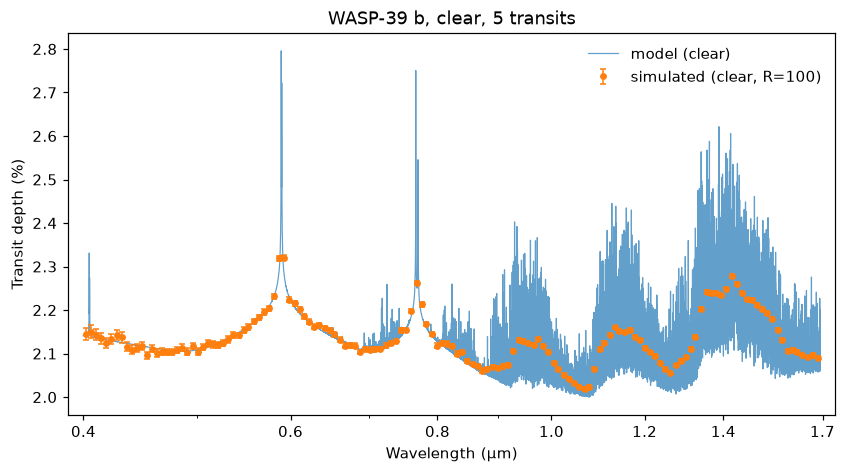
obs.plot() draws the native-resolution model as a line and one noisy realization of the binned spectrum as points with error bars. seed picks the realization; units is "percent" (default), "ppm" or "fraction".

obs.plot(seed=0)

Overlaying scenarios

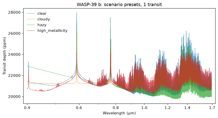
Pass the same ax to several calls. show_points=False draws only the model lines, and the legend entry is the scenario (or label if given). A title is set only on a new figure or an empty Axes, so set your own after an overlay.

fig, ax = plt.subplots(figsize=(9, 4.5))
for s in ["clear", "cloudy", "hazy", "high_metallicity"]:
    lazuli_exo.observe("WASP-39 b", scenario=s).plot(ax=ax, show_points=False, units="ppm")
ax.set_title("WASP-39 b: scenario presets, 1 transit")

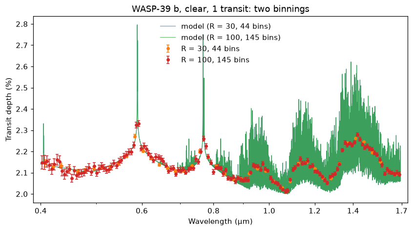
Two observations with points can share an Axes as well; label names the points and the matching model line (model (<label>)).

fig, ax = plt.subplots(figsize=(9, 4.5))
for R in (30, 100):
    o = lazuli_exo.observe("WASP-39 b", scenario="clear", R=R)
    o.plot(ax=ax, label=f"R = {R}, {o.wavelength.size} bins")
ax.set_title("WASP-39 b, clear, 1 transit: two binnings")

The error bar against wavelength

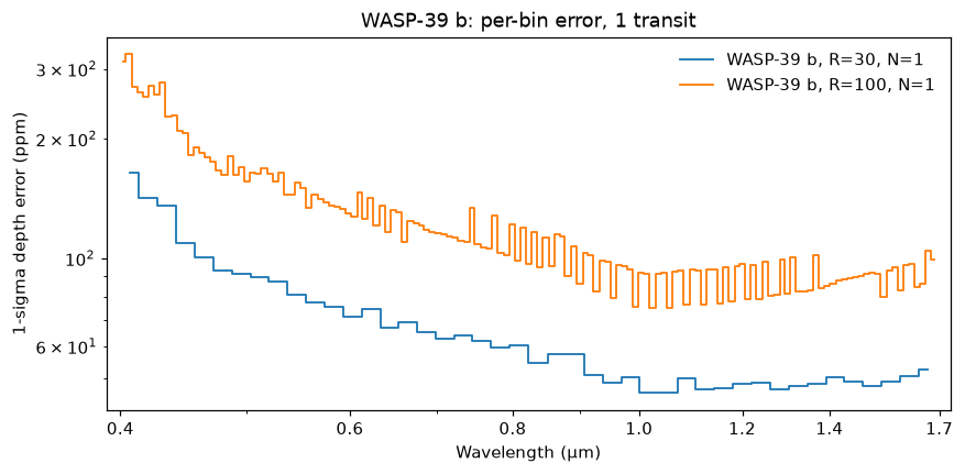
obs.plot_noise() shows where the instrument is precise: the per-bin 1-sigma uncertainty, with n_transits included, on a log scale. Overlay several binnings or transit counts to compare them directly.

fig, ax = plt.subplots(figsize=(9, 4))
for R in (30, 100):
    lazuli_exo.observe("WASP-39 b", R=R).plot_noise(ax=ax)
ax.set_title("WASP-39 b: per-bin error, 1 transit")

Light curves

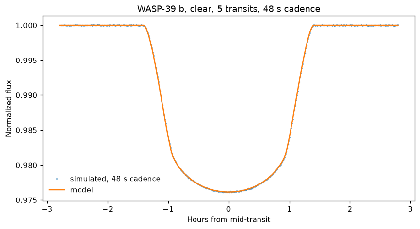
obs.light_curves(n_groups=1) is the white-light transit; its plot() draws the noisy samples and the noiseless model with a legend.

obs.light_curves(n_groups=1, seed=0).plot()

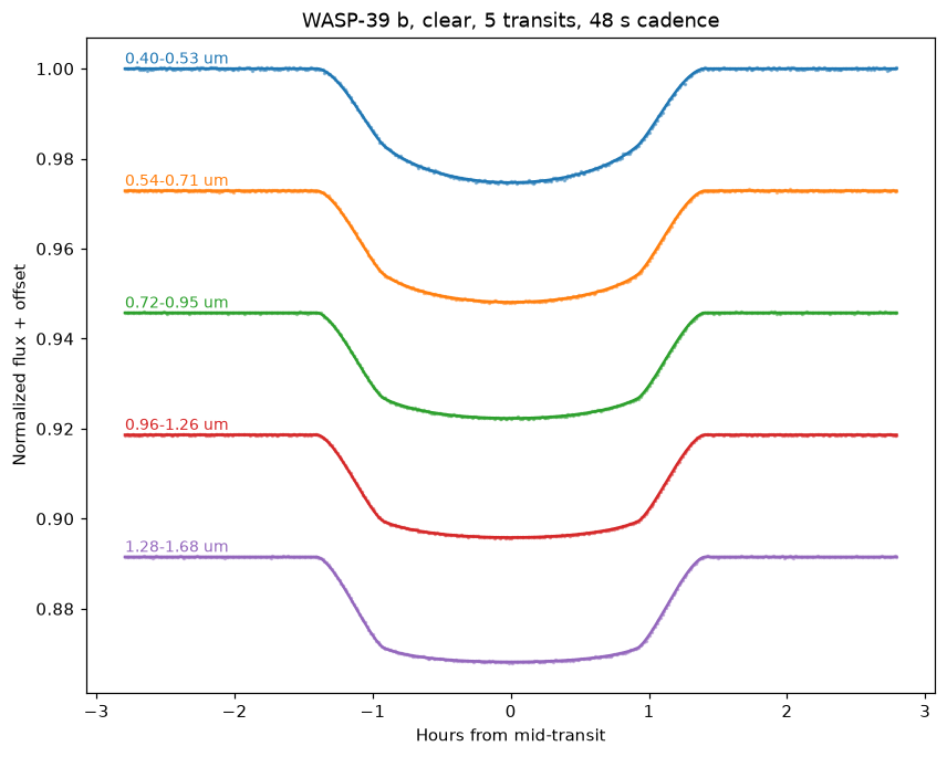
With several bands the curves stack, offset apart, each annotated with its wavelength range. The depth and the limb darkening change from band to band; the geometry is shared.

obs.light_curves(n_groups=5, seed=0).plot()

Tiling

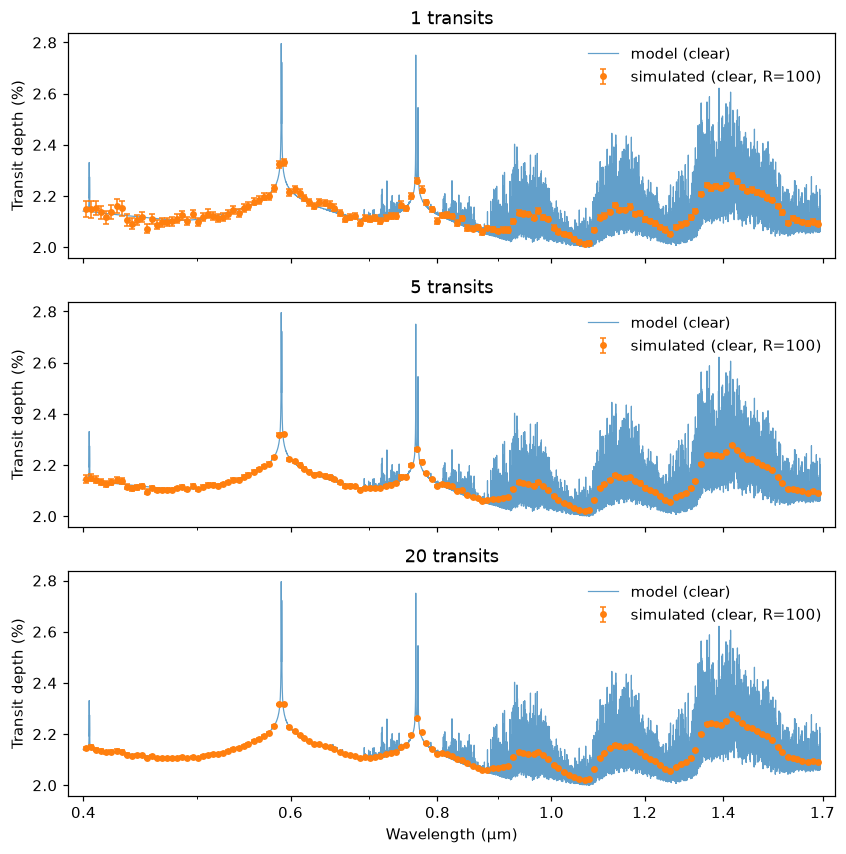
Because each call draws on the Axes you give it, a subplot grid works the same way. Shared x axes keep one wavelength range across the panels.

fig, axes = plt.subplots(3, 1, figsize=(9, 9), sharex=True)
for ax, n in zip(axes, (1, 5, 20)):
    lazuli_exo.observe("WASP-39 b", n_transits=n).plot(ax=ax, seed=0, title=f"{n} transits")
for ax in axes[:-1]:
    ax.set_xlabel("")

Keywords

Method	Keywords
`obs.plot`	`ax`, `seed`, `show_model`, `show_points`, `units`, `label`, `title`; anything else goes to `ax.errorbar` (`color` or `c` also colours the model line).
`obs.plot_noise`	`ax`, `units`, `label`; anything else goes to `ax.plot`.
`lc.plot`	`ax`, `offset` (band spacing in normalized flux), `show_points`, `show_model`, `label` (white light only), `title`.
`plotting.wavelength_axis(ax)`	Log wavelength axis with the Lazuli band ticks; call it after plotting on an Axes you drew yourself.