Note

This page is generated from the Jupyter notebook notebooks/02_verification.ipynb in the repository. You can download it and run it interactively.

Verifying the simulated images

The images from notebook 01 should behave like frames from the real instrument model. This notebook checks that they do: star centroids land where the WCS says, aperture photometry closes on the ETC count rates, source-free pixels follow the analytic noise model, bright stars are flagged as saturated, and the FITS output round-trips. Every section ends in an assertion, so the notebook doubles as a smoke test of the pipeline.

Requirements: a kernel with wcc_etc, wcc_sim and astroquery installed. The Gaia query is cached in gaia_cache/ (shared with notebook 01), so after the first run it works offline.

import numpy as np
import matplotlib.pyplot as plt
from astropy.io import fits

import wcc_etc
import wcc_sim
from wcc_sim import simulate_field

from wcc_sim.plotting import use_style, TEAL, RED, AMBER
use_style()

print(f'wcc_sim {wcc_sim.__version__} | wcc_etc {wcc_etc.__version__}')

wcc_sim 0.1.0 | wcc_etc 0.1.0

1. The test field

The same pointing, sensor and exposure as notebook 01: the full IMX455 array at (291.0, 44.5) in zwo:r, 90 s, in focus. We also keep a 600 x 600 px subarray centred on a bright, isolated, unsaturated star at each of the three focus levels; the astrometric and photometric checks below use it to measure the PSF without neighbours.

RA0, DEC0 = 291.0, 44.5   # deg, ICRS (Kepler field)
EXPTIME = 90.0             # s

field = simulate_field(
    ra=RA0, dec=DEC0, sensorfilter='zwo:r', focus=0,
    exptime=EXPTIME, seed=42, mag_limit=21.0,
    cache_dir='gaia_cache',
)

p = field.params
print(f"{p['n_sources']} Gaia sources (G <= {p['mag_limit']}), "
      f"{int(field.saturation_mask.sum())} saturated px")
print(f"plate scale {p['plate_scale_mas']:.2f} mas/px | sky {p['sky_e_s']:.3f} + "
      f"dark {p['dark_e_s']:.4f} e-/s/px | read noise {p['read_noise']:.2f} e- | "
      f"gain {p['gain']:.3f} e-/ADU")

img = field.image_adu
cat = field.catalog
inside = np.asarray(cat['in_image'], dtype=bool)
bg = (p['sky_e_s'] + p['dark_e_s']) * EXPTIME      # expected background per pixel [e-]
print(f'{inside.sum()} of {len(cat)} catalog stars land on the array')

100 Gaia sources (G <= 21.0), 167 saturated px
plate scale 16.87 mas/px | sky 0.014 + dark 0.0031 e-/s/px | read noise 3.04 e- | gain 0.261 e-/ADU
50 of 100 catalog stars land on the array

from scipy.spatial import cKDTree

xy = np.c_[cat['x'], cat['y']]
tree = cKDTree(xy)
neigh = tree.query(xy, k=2)[0][:, 1]                  # distance to nearest neighbor [px]
sat = np.asarray(cat['saturated'], dtype=bool)
ok = inside & ~sat & (neigh > 180)                    # isolated: > 3 arcsec
star = cat[ok][np.argmin(cat['phot_g_mean_mag'][ok])]
print(f"star: Gaia DR3 {star['source_id']}  G={star['phot_g_mean_mag']:.2f}  "
      f"spt={star['spt']}  rate={star['rate_e_s']:.0f} e-/s")

fields_focus = {}
for foc in (0, 1, 2):
    fields_focus[foc] = simulate_field(
        ra=float(star['ra']), dec=float(star['dec']), sensorfilter='zwo:r',
        focus=foc, exptime=EXPTIME, seed=42, shape=(600, 600),
        cache_dir='gaia_cache',
    )
print('subarray sims done')

star: Gaia DR3 2126245588779207936  G=18.26  spt=G5V  rate=1912 e-/s

/Users/gudmundurstefansson/Dropbox/mypylib/notebooks/GIT/wcc-sim/src/wcc_sim/psf.py:35: RuntimeWarning: divide by zero encountered in matmul
  cx = (psf.sum(axis=0) @ i) / total
/Users/gudmundurstefansson/Dropbox/mypylib/notebooks/GIT/wcc-sim/src/wcc_sim/psf.py:35: RuntimeWarning: overflow encountered in matmul
  cx = (psf.sum(axis=0) @ i) / total
/Users/gudmundurstefansson/Dropbox/mypylib/notebooks/GIT/wcc-sim/src/wcc_sim/psf.py:35: RuntimeWarning: invalid value encountered in matmul
  cx = (psf.sum(axis=0) @ i) / total
/Users/gudmundurstefansson/Dropbox/mypylib/notebooks/GIT/wcc-sim/src/wcc_sim/psf.py:36: RuntimeWarning: divide by zero encountered in matmul
  cy = (psf.sum(axis=1) @ i) / total
/Users/gudmundurstefansson/Dropbox/mypylib/notebooks/GIT/wcc-sim/src/wcc_sim/psf.py:36: RuntimeWarning: overflow encountered in matmul
  cy = (psf.sum(axis=1) @ i) / total
/Users/gudmundurstefansson/Dropbox/mypylib/notebooks/GIT/wcc-sim/src/wcc_sim/psf.py:36: RuntimeWarning: invalid value encountered in matmul
  cy = (psf.sum(axis=1) @ i) / total
/Users/gudmundurstefansson/Dropbox/mypylib/notebooks/GIT/wcc-sim/src/wcc_sim/psf.py:35: RuntimeWarning: divide by zero encountered in matmul
  cx = (psf.sum(axis=0) @ i) / total
/Users/gudmundurstefansson/Dropbox/mypylib/notebooks/GIT/wcc-sim/src/wcc_sim/psf.py:35: RuntimeWarning: overflow encountered in matmul
  cx = (psf.sum(axis=0) @ i) / total
/Users/gudmundurstefansson/Dropbox/mypylib/notebooks/GIT/wcc-sim/src/wcc_sim/psf.py:35: RuntimeWarning: invalid value encountered in matmul
  cx = (psf.sum(axis=0) @ i) / total
/Users/gudmundurstefansson/Dropbox/mypylib/notebooks/GIT/wcc-sim/src/wcc_sim/psf.py:36: RuntimeWarning: divide by zero encountered in matmul
  cy = (psf.sum(axis=1) @ i) / total
/Users/gudmundurstefansson/Dropbox/mypylib/notebooks/GIT/wcc-sim/src/wcc_sim/psf.py:36: RuntimeWarning: overflow encountered in matmul
  cy = (psf.sum(axis=1) @ i) / total
/Users/gudmundurstefansson/Dropbox/mypylib/notebooks/GIT/wcc-sim/src/wcc_sim/psf.py:36: RuntimeWarning: invalid value encountered in matmul
  cy = (psf.sum(axis=1) @ i) / total

subarray sims done

2. PSF modes: peak ordering

Defocus spreads a star’s light over more pixels, so the peak pixel must fall from in focus to +1 wave to +2 waves. The radial profiles of the noiseless subarrays show the Airy core and the two rings.

from wcc_sim.plotting import plot_radial_profile

bg = (p['sky_e_s'] + p['dark_e_s']) * EXPTIME
fig, ax = plt.subplots(figsize=(7.5, 5))
for foc, col, lab in [(0, TEAL, 'in focus'), (1, RED, '+1 wave'), (2, AMBER, '+2 waves')]:
    f = fields_focus[foc]
    row = int(np.flatnonzero(f.catalog['source_id'] == star['source_id'])[0])
    plot_radial_profile(f.image_clean, float(f.catalog['x'][row]), float(f.catalog['y'][row]),
                        ax=ax, bg=bg, r_max=160, color=col, label=lab)
ax.set_ylabel('mean profile [e$^-$/px]')
ax.set_title('Radial profiles of the noiseless image (16.87 mas/px)')
plt.show()

peak = {f: fields_focus[f].image_clean.max() - bg for f in (0, 1, 2)}
print(f"peak pixel: in-focus {peak[0]:.0f} e- | +1w {peak[1]:.0f} e- ({peak[1]/peak[0]:.1%}) "
      f"| +2w {peak[2]:.0f} e- ({peak[2]/peak[0]:.1%})")
assert peak[0] > peak[1] > peak[2], 'defocus must lower the peak'
print('PASS: peak ordering in-focus > +1w > +2w')

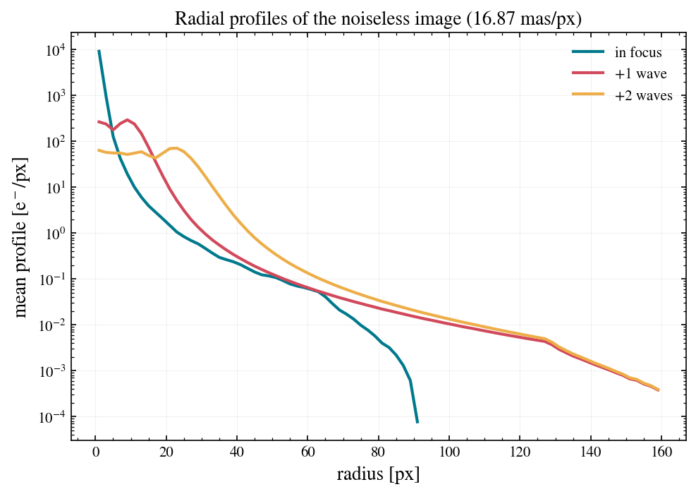
peak pixel: in-focus 14158 e- | +1w 308 e- (2.2%) | +2w 76 e- (0.5%)
PASS: peak ordering in-focus > +1w > +2w

3. Astrometry

Centroid the brightest isolated stars on the noiseless full-frame image and compare with the catalog positions predicted by the WCS. Sub-pixel placement uses an 11x oversampled PSF shift, so the quantization floor is 1/22 px, about 0.8 mas; centroids should agree to a few mas.

from photutils.centroids import centroid_com

sel = cat[ok]
sel = sel[np.argsort(sel['phot_g_mean_mag'])][:15]     # 15 brightest isolated stars
clean = field.image_clean
h = 20
resid_mas = []
for s in sel:
    x0, y0 = int(round(s['x'])), int(round(s['y']))
    if not (h < x0 < clean.shape[1] - h and h < y0 < clean.shape[0] - h):
        continue
    cut = clean[y0 - h:y0 + h + 1, x0 - h:x0 + h + 1] - bg
    cx, cy = centroid_com(np.clip(cut, 0, None))
    resid_mas.append(((x0 - h + cx) - s['x']) * 16.87), resid_mas.append(((y0 - h + cy) - s['y']) * 16.87)

resid_mas = np.array(resid_mas)
rms = np.sqrt(np.mean(resid_mas ** 2))

fig, ax = plt.subplots(figsize=(7, 4.5))
ax.hist(resid_mas, bins=15, color=TEAL, alpha=0.85)
ax.axvline(0, color='0.4', ls='--')
ax.set_xlabel('centroid $-$ catalog position [mas]'); ax.set_ylabel('N')
ax.set_title(f'Astrometric residuals: RMS = {rms:.2f} mas (plate scale 16.87 mas/px)')
plt.show()

assert rms < 10, f'astrometric RMS too large: {rms:.2f} mas'
print(f'PASS: astrometric RMS {rms:.2f} mas < 10 mas')

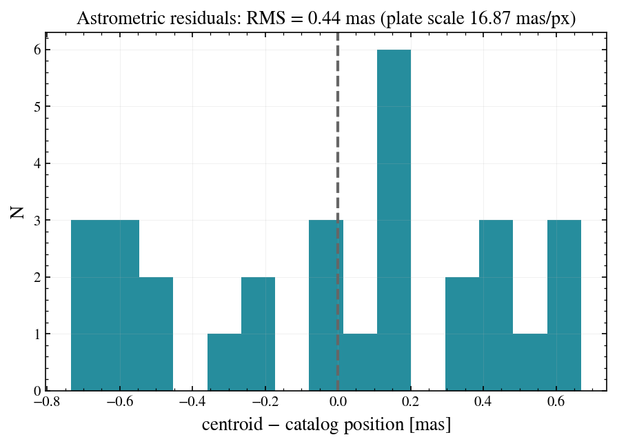
PASS: astrometric RMS 0.44 mas < 10 mas

4. Photometric closure

Aperture photometry (r = 40 px, annulus background) on both the noiseless and the noisy image, compared with each star’s expected flux rate_e_s x exptime from the ETC chain times the fraction of the PSF the aperture captures. That fraction is measured the same way on the noiseless in-focus subarray of section 1: the diffraction wings and the scattered-light halo put a few percent of every star’s light beyond 40 px, so a raw aperture sum does not close on the total rate. With the aperture fraction taken out, the noiseless measurements should close to about 1% and the noisy scatter should stay inside the propagated noise envelope.

from photutils.aperture import CircularAnnulus, CircularAperture, aperture_photometry

R_AP, R_IN, R_OUT = 40, 60, 90
m = ok & (cat['x'] > R_OUT) & (cat['x'] < img.shape[1] - R_OUT) \
       & (cat['y'] > R_OUT) & (cat['y'] < img.shape[0] - R_OUT)
stars = cat[m]
pos = np.c_[stars['x'], stars['y']]
aper, ann = CircularAperture(pos, r=R_AP), CircularAnnulus(pos, r_in=R_IN, r_out=R_OUT)

def measure(image):
    phot = aperture_photometry(image, aper)
    bkg = aperture_photometry(image, ann)['aperture_sum'] / ann.area
    return np.asarray(phot['aperture_sum'] - bkg * aper.area)

# aperture fraction of the model PSF: same aperture + annulus on the isolated star of section 1
sub = fields_focus[0]
xs, ys = float(sub.catalog['x'][sub.catalog['source_id'] == star['source_id']][0]), \
         float(sub.catalog['y'][sub.catalog['source_id'] == star['source_id']][0])
ap1, ann1 = CircularAperture((xs, ys), r=R_AP), CircularAnnulus((xs, ys), r_in=R_IN, r_out=R_OUT)
flux1 = (aperture_photometry(sub.image_clean, ap1)['aperture_sum'][0]
         - aperture_photometry(sub.image_clean, ann1)['aperture_sum'][0] / ann1.area * ap1.area)
ee_ap = float(flux1 / (star['rate_e_s'] * EXPTIME))
print(f'aperture fraction at r = {R_AP} px: {ee_ap:.4f}')

expected = np.asarray(stars['rate_e_s']) * EXPTIME * ee_ap
meas_clean = measure(field.image_clean)
meas_noisy = measure(field.image_e)

resid_clean = 100 * (meas_clean - expected) / expected
resid_noisy = 100 * (meas_noisy - expected) / expected
npix = np.pi * R_AP ** 2
sigma_pct = 100 * np.sqrt(expected + npix * bg + npix * p['read_noise'] ** 2) / expected

g = np.asarray(stars['phot_g_mean_mag'])
fig, axes = plt.subplots(1, 2, figsize=(12.5, 4.6))
axes[0].loglog(expected, meas_clean, 'o', color=TEAL, ms=5)
lims = [expected.min() * 0.5, expected.max() * 2]
axes[0].plot(lims, lims, color='0.4', ls='--', lw=1)
axes[0].set_xlabel('expected flux [e$^-$]'); axes[0].set_ylabel('measured flux [e$^-$]')
axes[0].set_title('Noiseless image: measured vs ETC expectation')

order = np.argsort(g)
axes[1].plot(g, resid_noisy, 'o', color=RED, ms=4, label='noisy image')
axes[1].plot(g, resid_clean, 'o', color=TEAL, ms=4, label='noiseless image')
axes[1].plot(g[order], 3 * sigma_pct[order], color='0.4', ls='--', lw=1, label=r'$\pm3\sigma$ (photon+sky+read)')
axes[1].plot(g[order], -3 * sigma_pct[order], color='0.4', ls='--', lw=1)
axes[1].set_xlabel('Gaia G [mag]'); axes[1].set_ylabel('residual [%]')
axes[1].set_title('Photometric residuals vs G')
axes[1].legend()
plt.show()

med = np.median(np.abs(resid_clean))
frac_in = np.mean(np.abs(resid_noisy) < 3 * sigma_pct)
print(f'noiseless closure: median |resid| = {med:.2f}%  (n={len(stars)})')
print(f'noisy photometry: {100*frac_in:.0f}% of stars within 3 sigma of expectation')
assert med < 2.0, 'noiseless closure worse than 2%'
assert frac_in > 0.9, 'too many noisy measurements outside 3 sigma'
print('PASS: photometry closes on the ETC prediction')

aperture fraction at r = 40 px: 0.9796

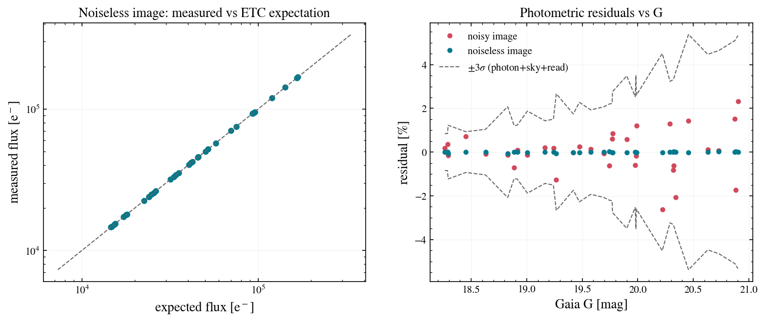
noiseless closure: median |resid| = 0.01%  (n=34)
noisy photometry: 100% of stars within 3 sigma of expectation
PASS: photometry closes on the ETC prediction

5. Noise statistics

A source-free simulation should be pure sky, dark and read noise: pixel variance equal to (sky + dark) t + RN^2, with a near-Gaussian histogram at these count levels.

from astropy.table import Table
from wcc_sim.catalog import _empty_table

sky_field = simulate_field(ra=RA0, dec=DEC0, sensorfilter='zwo:r', focus=0,
                           exptime=EXPTIME, seed=7, shape=(512, 512),
                           catalog=_empty_table())
pix = sky_field.image_e.ravel()
lam = (p['sky_e_s'] + p['dark_e_s']) * EXPTIME
var_exp = lam + p['read_noise'] ** 2

fig, ax = plt.subplots(figsize=(7.5, 4.8))
ax.hist(pix, bins=100, density=True, color=TEAL, alpha=0.85, label='sky-only pixels')
xx = np.linspace(pix.min(), pix.max(), 400)
ax.plot(xx, np.exp(-(xx - lam) ** 2 / (2 * var_exp)) / np.sqrt(2 * np.pi * var_exp),
        color=RED, label=r'Gaussian: $\mu=(sky+dark)\,t$, $\sigma^2=\mu+RN^2$')
ax.set_xlabel('pixel value [e$^-$]'); ax.set_ylabel('density')
ax.set_title('Source-free image vs analytic noise model')
ax.legend()
plt.show()

print(f'mean: measured {pix.mean():.2f} vs expected {lam:.2f} e-')
print(f'var : measured {pix.var():.2f} vs expected {var_exp:.2f} e-^2')
assert abs(pix.mean() - lam) < 0.05 * max(lam, 1), 'mean off'
assert abs(pix.var() - var_exp) < 0.10 * var_exp, 'variance off'
print('PASS: noise statistics match (sky+dark)*t + RN^2')

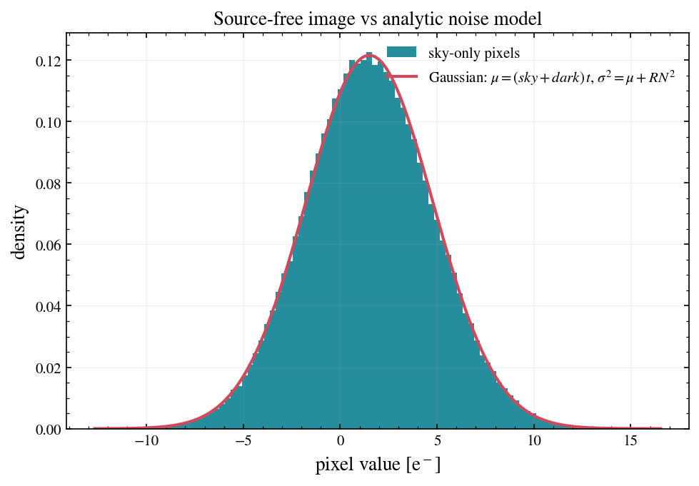
mean: measured 1.50 vs expected 1.50 e-
var : measured 10.79 vs expected 10.77 e-^2
PASS: noise statistics match (sky+dark)*t + RN^2

6. Saturation flags

Bright stars overfill the detector wells. The pipeline flags the affected pixels in the SATMASK extension and each affected star in the catalog. plot_image() works on any array; here it shows a cutout of the ADU image around the brightest saturated star with the matching slice of the mask drawn as a contour.

from wcc_sim.plotting import plot_image

sat_stars = cat[np.asarray(cat['saturated'], dtype=bool) & inside]
if len(sat_stars):
    s = sat_stars[np.argmin(sat_stars['phot_g_mean_mag'])]
    x0, y0 = int(round(s['x'])), int(round(s['y']))
    h = 60
    sl = np.s_[max(y0-h,0):y0+h, max(x0-h,0):x0+h]
    ax = plot_image(field.image_adu[sl], satmask=field.saturation_mask[sl], percent=99.9)
    ax.set_title(f"G={s['phot_g_mean_mag']:.1f} star, saturated pixels outlined")
    plt.show()
    print(f"{len(sat_stars)} saturated stars in frame; brightest G={s['phot_g_mean_mag']:.2f}")
else:
    print('no saturated stars in this field/exptime')

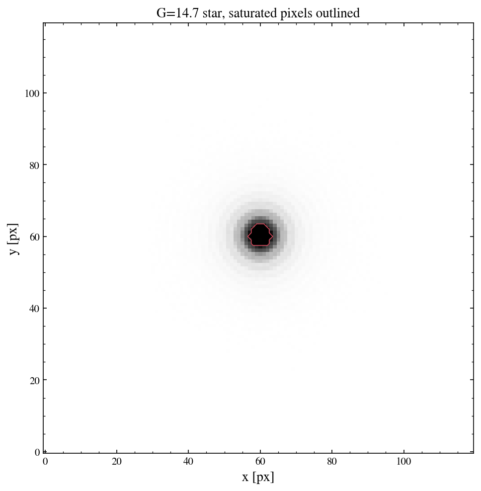
14 saturated stars in frame; brightest G=14.71

7. FITS round trip

The multi-extension file written by field.write() must come back with its four extensions, and the catalog table must hold as many rows as the NSRC header card says.

import os, tempfile

path = os.path.join(tempfile.mkdtemp(), 'field_1wave.fits')
fields_focus[1].write(path)
with fits.open(path) as f_check:
    names = [h.name for h in f_check]
    n_cat = len(f_check['CAT'].data)
    hdr = f_check['SCI'].header
print('extensions:', names)
print(f"CAT rows {n_cat} | NSRC card {hdr['NSRC']} | WCS {hdr['CTYPE1']}, {hdr['CTYPE2']}")
assert names == ['SCI', 'SATMASK', 'CAT', 'CLEAN']
assert n_cat == hdr['NSRC']
print('PASS: FITS output round-trips (SCI/SATMASK/CAT/CLEAN)')

extensions: ['SCI', 'SATMASK', 'CAT', 'CLEAN']
CAT rows 7 | NSRC card 7 | WCS RA---TAN, DEC--TAN
PASS: FITS output round-trips (SCI/SATMASK/CAT/CLEAN)

Summary

Verified in this notebook:

1. PSF modes: the in-focus Airy and the +1/+2-wave Huygens defocus PSFs render with the expected peak ordering and ring structure.

2. Astrometry: star centroids match the Gaia/WCS positions to a few-mas RMS.

3. Photometry: aperture fluxes close on the ETC rate x t prediction to about 1% (noiseless) and scatter within the propagated noise envelope (noisy).

4. Noise: source-free pixels follow mean = (sky + dark) t and variance = mean + RN^2.

5. Saturation and FITS: bright stars are flagged in SATMASK and CAT, and the multi-extension FITS output round-trips.

The ETC-versus-simulation cross-check also runs as a slow test in the test suite (pytest -m slow). The plots came from field.plot_cutout(), plot_radial_profile() and plot_image(); notebook 10 shows the rest of the plotting methods.