Note

This page is generated from the Jupyter notebook notebooks/07_cli_and_fits.ipynb in the repository. You can download it and run it interactively.

The command line and the FITS output

Everything simulate_field does is also available from the shell as wcc-sim. This notebook runs the CLI on a real Gaia pointing (cached in gaia_cache/, so it works offline) and dissects the multi-extension FITS file it writes.

Requirements: a kernel with wcc_etc, wcc_sim and astroquery installed.

[1]:

import numpy as np
import matplotlib.pyplot as plt

import wcc_etc
import wcc_sim

from wcc_sim.plotting import use_style, TEAL, RED, AMBER
use_style()

print(f'wcc_sim {wcc_sim.__version__} | wcc_etc {wcc_etc.__version__}')

import subprocess
import sys

def run(args):
    r = subprocess.run([sys.executable, '-m', 'wcc_sim.cli'] + args,
                       capture_output=True, text=True)
    print(r.stdout or r.stderr)
    assert r.returncode == 0, r.stderr
    return r

wcc_sim 0.1.0 | wcc_etc 0.1.0

1. `wcc-sim --help`

[2]:

run(['--help']);

usage: wcc-sim [-h] --ra RA --dec DEC [--sensorfilter SENSORFILTER]
               [--focus {0,1,2}] [--exptime EXPTIME] [--n-reads N_READS]
               [--pa PA] [--jitter JITTER_SIGMA_MAS] [--mag-limit MAG_LIMIT]
               [--no-noise] [--no-clean] [--seed SEED] [--shape NY NX]
               [--stamp-npix STAMP_NPIX] [--no-wings]
               [--wavelength WAVELENGTH_NM] [--report REPORT] [--no-scatter]
               [--scatter-fraction SCATTER_FRACTION] [--cache-dir CACHE_DIR]
               [--gain-mode GAIN_MODE] -o OUTPUT

Simulate a WCC detector image of the Gaia field at (RA, Dec).

options:
  -h, --help            show this help message and exit
  --ra RA               pointing RA [deg, ICRS]
  --dec DEC             pointing Dec [deg, ICRS]
  --sensorfilter SENSORFILTER
                        wcc_etc sensorfilter, e.g. zwo:r, zwo:r+1, qcmos:bb
  --focus {0,1,2}       waves of defocus (default: sensorfilter's focus level)
  --exptime EXPTIME     total exposure [s]
  --n-reads N_READS     coadded frames
  --pa PA               position angle [deg E of N]
  --jitter JITTER_SIGMA_MAS
                        jitter sigma [mas]
  --mag-limit MAG_LIMIT
                        Gaia G faint limit
  --no-noise            skip noise realization
  --no-clean            omit CLEAN extension
  --seed SEED           RNG seed (default: drawn at random and recorded as
                        SEED)
  --shape NY NX         subarray shape (default: full array)
  --stamp-npix STAMP_NPIX
                        PSF stamp size [detector px, odd]
  --no-wings            skip the analytic PSF wing extension beyond the stamp
  --wavelength WAVELENGTH_NM
                        wavelength for the Airy core [nm] (PSF geometry only;
                        default: the sensorfilter's central wavelength)
  --report REPORT       write a PDF+PNG PSF radial-profile report (Airy vs
                        scattered-light terms) to this path
  --no-scatter          skip the measured scattered-light halo (FRED stray
                        light); implied by --no-wings
  --scatter-fraction SCATTER_FRACTION
                        instrument-wide scattered fraction (default: FRED's
                        F_FOCAL, 7.13e-3)
  --cache-dir CACHE_DIR
                        Gaia query cache directory
  --gain-mode GAIN_MODE
                        readout gain mode for multi-mode detectors (qcmos:
                        'high' = 32x, clips at 552 e-; 'low' = 1x)
  -o, --output OUTPUT   output FITS path

2. Simulate a field from the shell

A 600×600 px cutout of a Kepler-field pointing at +1 wave defocus. --cache-dir gaia_cache reuses the cone search shipped with the repository, so no network is needed; --seed pins the noise realization.

[3]:

run(['--ra', '291.017019', '--dec', '44.495843',
     '--sensorfilter', 'zwo:r', '--focus', '1',
     '--exptime', '90', '--seed', '42',
     '--shape', '600', '600', '--cache-dir', 'gaia_cache',
     '-o', 'cli_field_1wave.fits']);

Wrote cli_field_1wave.fits: 600x600 px, 7 sources, focus=1w, scatter=on, 0 saturated px

3. What is in the file

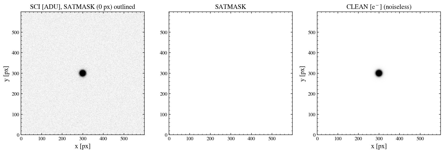
Four extensions: the ADU image (SCI, with WCS + provenance header), the per-pixel saturation mask (SATMASK), the injected catalog (CAT), and the noiseless expectation image (CLEAN, omit with --no-clean). plot_image() from wcc_sim.plotting takes the raw arrays read back from the file, so no SimulatedField is needed to look at them.

[4]:

from astropy.io import fits

hdul = fits.open('cli_field_1wave.fits')
hdul.info()

Filename: cli_field_1wave.fits
No.    Name      Ver    Type      Cards   Dimensions   Format
  0  SCI           1 PrimaryHDU      65   (600, 600)   float32
  1  SATMASK       1 ImageHDU         8   (600, 600)   uint8
  2  CAT           1 BinTableHDU     54   7R x 18C   [K, D, D, E, E, E, D, D, D, E, D, D, 3A, L, D, D, L, L]
  3  CLEAN         1 ImageHDU         9   (600, 600)   float32

[5]:

hdr = hdul['SCI'].header
for card in ['RA_PNT', 'DEC_PNT', 'SENSORF', 'FOCUS', 'EXPTIME', 'NREADS',
             'JITTER', 'MAGLIM', 'SEED', 'NSRC', 'PLTSCL', 'GAIN', 'RDNOISE',
             'DARK', 'SKYRATE', 'WELLDEP', 'WCCSIMV', 'WCCETCV', 'BUNIT']:
    print(f'{card:8s} = {hdr[card]!r:>24}   / {hdr.comments[card]}')

RA_PNT   =               291.017019   / [deg] pointing RA (ICRS), array center
DEC_PNT  =                44.495843   / [deg] pointing Dec (ICRS), array center
SENSORF  =                  'zwo:r'   / wcc_etc sensorfilter (kind:band)
FOCUS    =                        1   / [waves] defocus (0=in-focus)
EXPTIME  =                     90.0   / [s] total exposure time
NREADS   =                        1   / coadded frames (ETC semantics)
JITTER   =                     10.0   / [mas] jitter Gaussian sigma
MAGLIM   =                     21.0   / Gaia G faint limit of injected sources
SEED     =                       42   / RNG seed (drawn at random if not given)
NSRC     =                        7   / number of injected sources
PLTSCL   =       16.869089722675366   / [mas/pix] plate scale
GAIN     =        0.261200000004368   / [e-/ADU] sensor gain
RDNOISE  =       3.0442890448219115   / [e-] read noise per frame
DARK     =     0.003070336749998594   / [e-/s/pix] dark current
SKYRATE  =     0.013643288040258746   / [e-/s/pix] sky background rate
WELLDEP  =       16274.929434794496   / [e-] full well (empty if None)
WCCSIMV  =                  '0.1.0'   / wcc_sim version
WCCETCV  =                  '0.1.0'   / wcc_etc version
BUNIT    =                    'adu'   / SCI pixel units

[6]:

from wcc_sim.plotting import plot_image

sci = hdul['SCI'].data
sat = hdul['SATMASK'].data.astype(bool)
clean = hdul['CLEAN'].data

fig, axes = plt.subplots(1, 3, figsize=(15, 4.6))
plot_image(sci, ax=axes[0], satmask=sat)
axes[0].set_title(f'SCI [ADU], SATMASK ({sat.sum()} px) outlined')
axes[1].imshow(sat, origin='lower', cmap='gray_r', interpolation='none')
axes[1].set_title('SATMASK'); axes[1].grid(False)
plot_image(clean, ax=axes[2])
axes[2].set_title('CLEAN [e$^-$] (noiseless)')
plt.show()

../_images/notebooks_07_cli_and_fits_9_0.png

4. The catalog extension

CAT carries every injected Gaia source with its pixel position, assigned spectral type, count rate, and flags: everything needed to evaluate photometry or train on the image.

[7]:

from astropy.table import Table

cat = Table.read(hdul['CAT'])
cat.sort('phot_g_mean_mag')
print(f'{len(cat)} sources | {np.asarray(cat["in_image"], bool).sum()} in frame | '
      f'{np.asarray(cat["saturated"], bool).sum()} flagged saturated')
cat[:8]

7 sources | 1 in frame | 0 flagged saturated

[7]:

Table length=7

source_id	ra	dec	phot_g_mean_mag	phot_bp_mean_mag	phot_rp_mean_mag	pmra	pmdec	parallax	radial_velocity	x	y	spt	spt_fallback	rate_e_s	psf_wavelength_nm	in_image	saturated
	deg	deg	mag	mag	mag	mas / yr	mas / yr	mas	km / s
int64	float64	float64	float32	float32	float32	float64	float64	float64	float32	float64	float64	str3	bool	float64	float64	bool	bool
2126245691858425728	291.0211043559742	44.4969746878879	16.742466	17.188572	16.14136	-2.120071545648841	-5.82184772669779	0.14562202596728072	--	-322.37821688720305	541.0268749834006	K0V	False	7845.448772406409	614.0257013294289	False	False
2126245687559826048	291.02327197511016	44.49729688452118	18.237642	18.737148	17.609856	0.6783309316902747	-0.8024744088834808	0.35604114156519634	--	-652.330771323393	609.8071028426876	K2V	False	2003.1463906702188	614.0257013294289	False	False
2126245588779207936	291.0170189106795	44.495842626555834	18.262655	18.628824	17.74546	-3.465808387452646	-5.304146474099873	0.13236246122923595	--	299.51359674851705	299.4203039963873	G5V	False	1912.1962074946161	614.0257013294289	True	False
2126245794937637632	291.01408663507874	44.4978801095047	18.886478	19.299976	18.357029	-2.459316322966642	-4.991159235076833	-0.05786958254748585	--	745.8614834546491	734.2436280732969	G8V	False	1084.7633569057168	614.0257013294289	False	False
2126245790639029504	291.0104300591018	44.49512296717736	19.576889	19.926746	19.043058	-2.4222883109058624	-5.0511992911369745	-0.40984207091909397	--	1302.5090313339151	145.87959946750735	G5V	False	569.9750170521618	614.0257013294289	False	False
2126245584480594432	291.01765804648454	44.493791125062245	19.900595	21.206516	18.84191	5.702391004604033	8.783545223866842	1.245635299861406	--	202.21819950324004	-138.3863048764921	M2V	False	272.73719294852356	614.0257013294289	False	False
2126245584477751168	291.0218141943379	44.49254029274426	20.22042	21.373112	19.00277	-2.2535144488758156	-3.3436176450148487	1.0528398238695984	--	-430.4862472893402	-405.3029976034127	M2V	False	202.3910015664441	614.0257013294289	False	False

5. Astrometric closure through the file

The WCS in the SCI header must map the catalog’s (ra, dec) back onto its stored pixel positions, a full round-trip through the FITS file.

[8]:

from astropy.wcs import WCS

wcs = WCS(hdr)
x, y = wcs.world_to_pixel_values(np.asarray(cat['ra'], float),
                                 np.asarray(cat['dec'], float))
err = np.hypot(x - cat['x'], y - cat['y']).max()
print(f'max |WCS(ra,dec) - (x,y)| = {err:.2e} px')
assert err < 1e-3
hdul.close()

max |WCS(ra,dec) - (x,y)| = 2.81e-12 px

Summary

wcc-sim exposes the whole pipeline from the shell; --cache-dir makes reruns offline and --seed makes them reproducible.
The FITS file is self-describing: WCS + full provenance in the SCI header, per-pixel SATMASK, the injected CAT, and a noiseless CLEAN image.
See the CLI page of the documentation for the full option table and a cookbook, and scripts/ for ready-to-run examples.