Note

This page is generated from the Jupyter notebook notebooks/10_plotting.ipynb in the repository. You can download it and run it interactively.

Plotting: every .plot_* method in one place

Every result object in wcc-sim and wcc-phot can draw itself. SimulatedField has plot(), plot_cutout(), plot_psf_profile() and plot_satmask(); PhotometryResult has plot(), plot_field(), plot_centroids() and the other panels of its diagnostic report. Each method takes ax=None: leave it out to get a new figure in the packaged house style, or pass an axes to draw into a figure of your own. Each returns the axes, so titles and limits can be adjusted afterwards.

The functions behind the methods live in wcc_sim.plotting (images, radial profiles, stamps, encircled energy), wcc_sim.psfreport (the PSF panels) and wcc_phot.report (the photometry panels). They work on plain arrays too, so an image read back from a FITS file can be shown the same way.

This notebook runs offline on a synthetic catalog: a G = 6 star that saturates and fourteen G = 18.6 to 20.5 stars around it, on a 1024 x 1024 subarray of the IMX455 in zwo:r. The faint stars sit just below the saturation limit: the IMX455 well holds only about 16 ke-, so at 60 s in focus anything brighter than G of about 18.5 saturates.

Requirements: a kernel with wcc_etc and wcc_sim installed.

import numpy as np
import matplotlib.pyplot as plt
from astropy.table import Table

import wcc_sim
import wcc_phot
from wcc_sim import simulate_field
from wcc_sim.detectors import get_geometry
from wcc_sim.wcsutil import build_wcs
from wcc_sim.plotting import use_style, TEAL, RED, AMBER

use_style()   # the packaged style, src/wcc_sim/data/plot_default.mplstyle
print(f'wcc_sim {wcc_sim.__version__} | wcc_phot {wcc_phot.__version__}')

wcc_sim 0.1.0 | wcc_phot 0.1.0

1. A synthetic field

The stars are laid out in pixel space and converted to sky coordinates through the same TAN WCS the simulator will build, so we know where each one lands. Row 0 of the catalog is the bright star, which is the row the PSF panels profile by default.

RA0, DEC0 = 150.1, 2.2
SHAPE = (1024, 1024)
EXPTIME = 60.0

geom = get_geometry('zwo:r')
w = build_wcs(RA0, DEC0, geom.plate_scale_mas, 0.0, SHAPE)
rng = np.random.default_rng(9)
n_faint = 14
x_px = np.concatenate([[512.0], rng.uniform(80, 944, n_faint)])
y_px = np.concatenate([[512.0], rng.uniform(80, 944, n_faint)])
gmag = np.concatenate([[6.0], rng.uniform(18.6, 20.5, n_faint)])
ras, decs = w.pixel_to_world_values(x_px, y_px)
cat = Table({
    'source_id': np.arange(gmag.size), 'ra': ras, 'dec': decs,
    'phot_g_mean_mag': gmag,
    'phot_bp_mean_mag': gmag + 0.4,   # BP - RP = 0.8, a G dwarf
    'phot_rp_mean_mag': gmag - 0.4,
})

field = simulate_field(RA0, DEC0, sensorfilter='zwo:r', focus=0, exptime=EXPTIME,
                       seed=1, catalog=cat, shape=SHAPE)
print(f"{field.params['n_sources']} stars, {int(field.saturation_mask.sum())} saturated px, "
      f"scatter halo {'on' if field.params['scatter'] else 'off'}")

15 stars, 3873 saturated px, scatter halo on

2. field.plot()

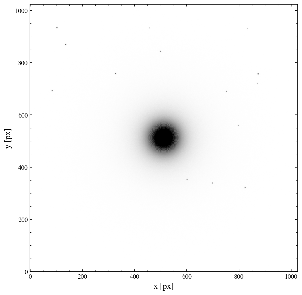
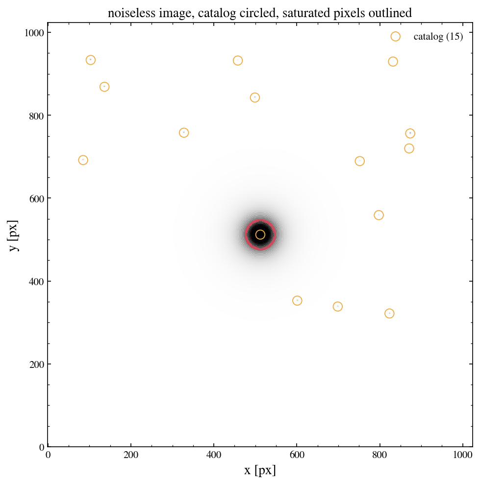
The delivered ADU image on an asinh stretch. which= switches to the electron image ('e') or the noiseless expectation ('clean'); catalog=True circles the stars that land on the array and satmask=True outlines the saturated pixels. A full 61 Mpix frame is reduced by block maximum for display (max_px sets the threshold) while the axes stay in native pixels.

field.plot();

ax = field.plot(which='clean', catalog=True, satmask=True)
ax.set_title('noiseless image, catalog circled, saturated pixels outlined');

3. field.plot_cutout()

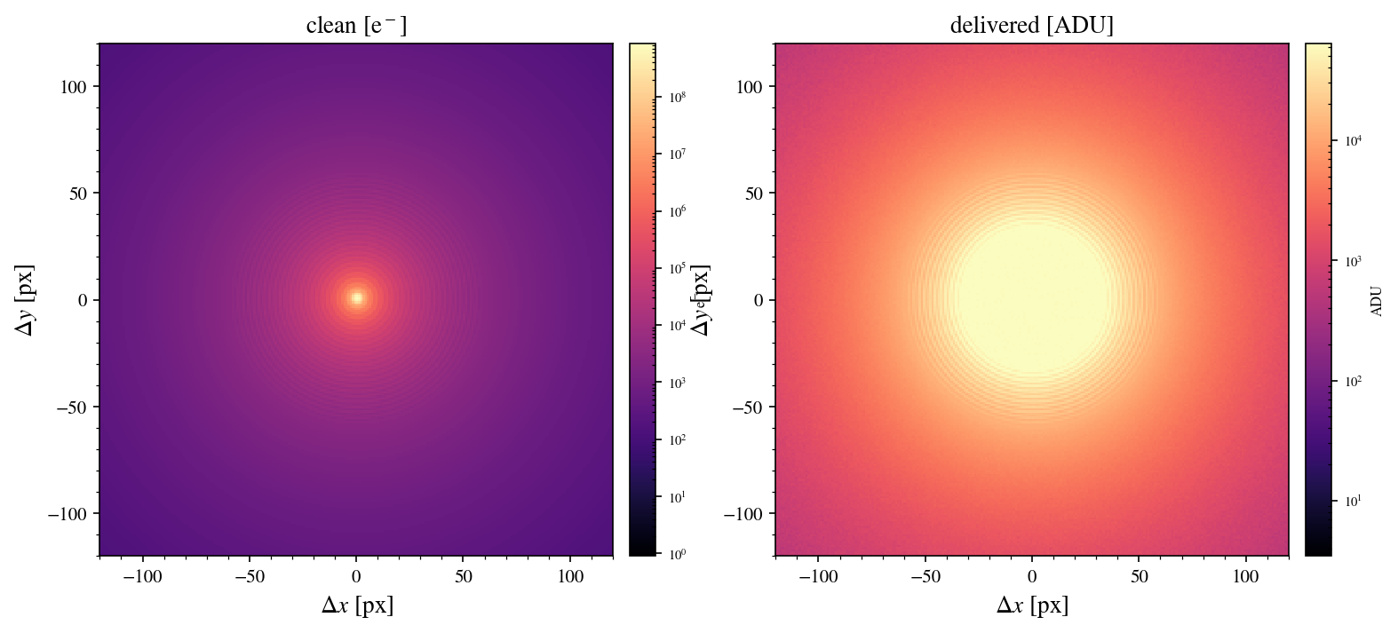
A cutout around one catalog row (star=, default 0) on a log stretch whose floor is the sky level, so the diffraction rings and the first part of the halo show. which= picks the image as above.

fig, axes = plt.subplots(1, 2, figsize=(12, 5))
field.plot_cutout(ax=axes[0], half_width=120)
field.plot_cutout(ax=axes[1], half_width=120, which='adu')
axes[0].set_title('clean [e$^-$]'); axes[1].set_title('delivered [ADU]');

4. field.plot_psf_profile()

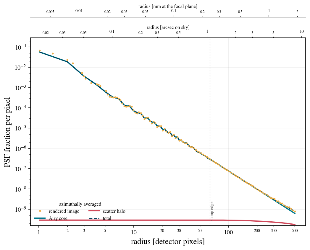
The azimuthally averaged radial profile of the bright star, split into the Airy core (with its fitted wing), the scattered-light halo, and their total, against what actually landed in the noiseless image. The vertical lines mark the stamp edge, the crossover where the halo overtakes the diffraction wing, and the radius to which the star was drawn. The same panel is the centrepiece of the PSF report.

field.plot_psf_profile();

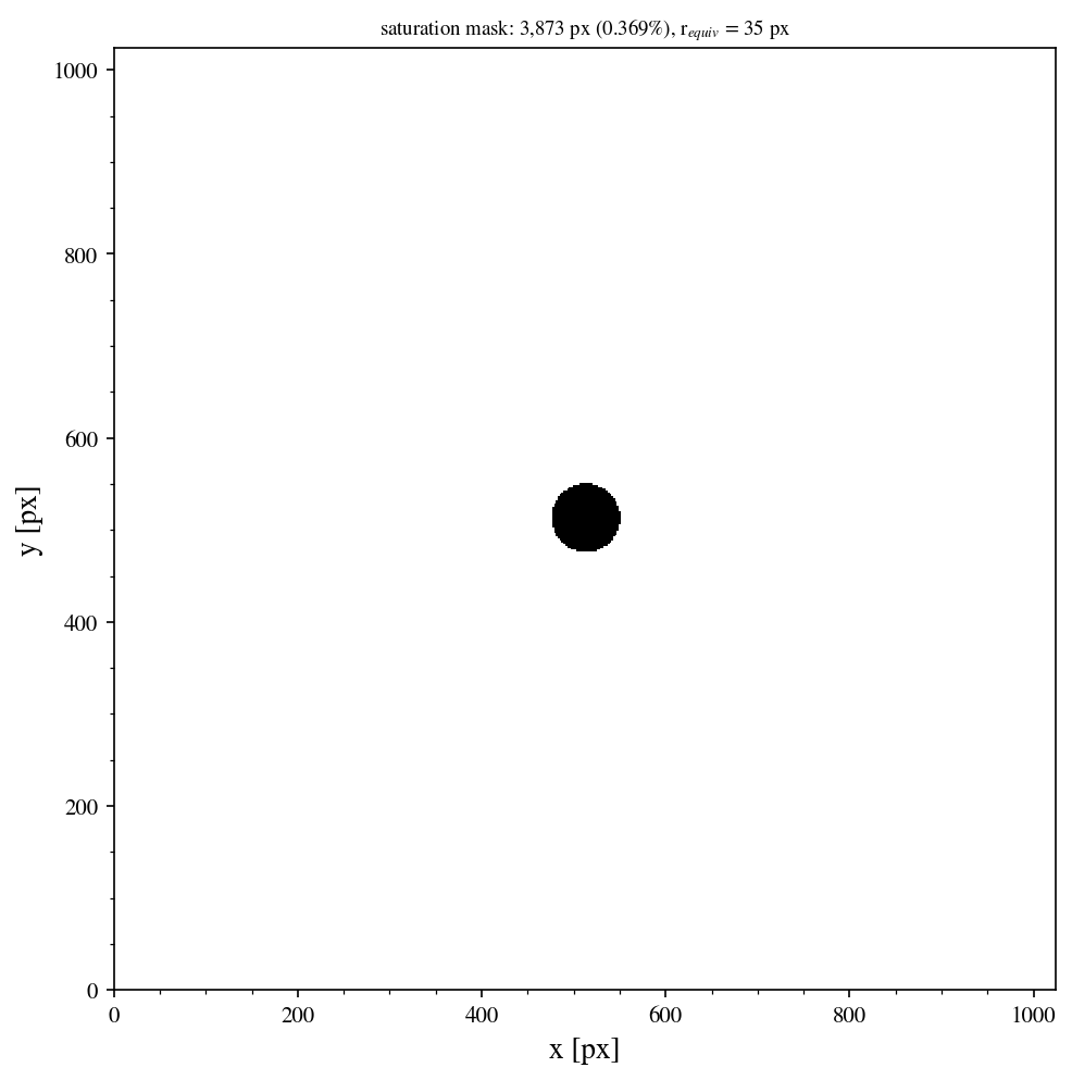
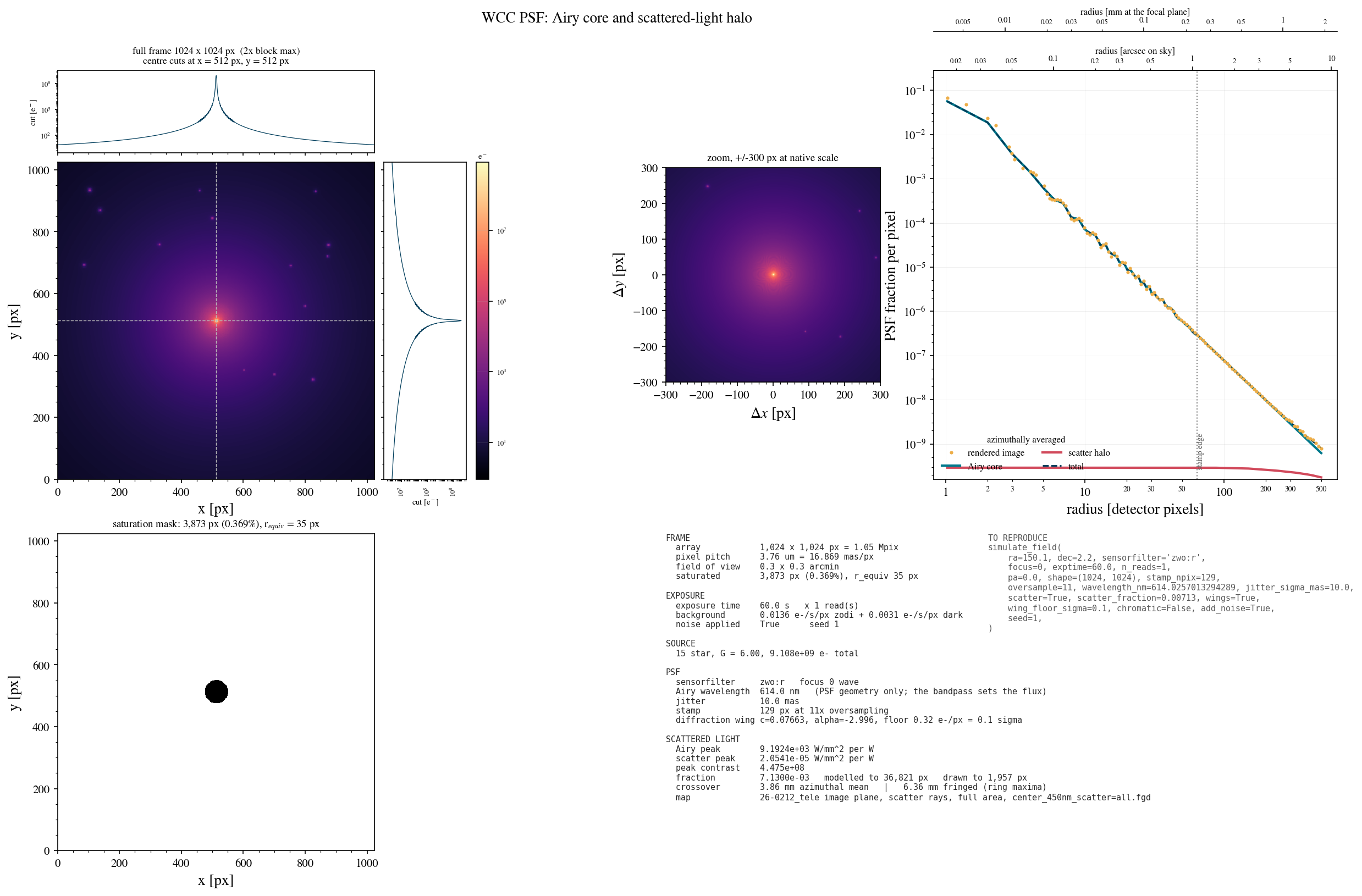
5. field.plot_satmask() and field.psf_report()

The saturation mask on its own, and the full one-page PSF report. psf_report(path) writes a PDF and a PNG and returns both paths; build_psf_figure() returns the figure itself, which is handy inside a notebook.

field.plot_satmask();

import tempfile, os
from wcc_sim.psfreport import build_psf_figure, psf_decomposition

outdir = tempfile.mkdtemp()
pdf, png = field.psf_report(os.path.join(outdir, 'psf_report.pdf'))
print('wrote', os.path.basename(pdf), 'and', os.path.basename(png))

dec = psf_decomposition(field)
print(f"Airy peak / scatter peak = {dec['contrast']:.2e}, "
      f"crossover at {dec['crossover_px']:.0f} px, drawn to {dec['r_out_px']:.0f} px")

fig, _ = build_psf_figure(field)
fig

wrote psf_report.pdf and psf_report.png
Airy peak / scatter peak = 4.48e+08, crossover at 1027 px, drawn to 1957 px

6. Stamps, radial profiles and encircled energy

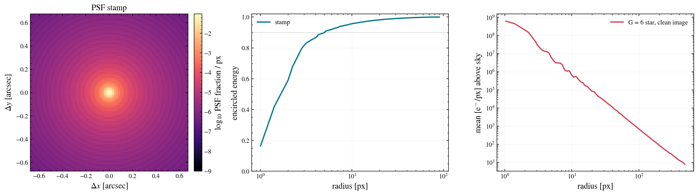
The functions in wcc_sim.plotting take arrays. field.models['stamp'] is the detector-sampled PSF stamp the render used; plot_stamp() shows it on a log colour scale (in arcsec when given a plate scale), plot_encircled_energy() the cumulative fraction inside each radius, and plot_radial_profile() the mean in annuli about any point of any image.

from wcc_sim.plotting import plot_stamp, plot_encircled_energy, plot_radial_profile

stamp = field.models['stamp']
fig, axes = plt.subplots(1, 3, figsize=(16, 4.4))
plot_stamp(stamp, ax=axes[0], half_width=40, plate_scale_mas=field.params['plate_scale_mas'],
           title='PSF stamp')
plot_encircled_energy(stamp, ax=axes[1], color=TEAL, label='stamp')
axes[1].axhline(0.9, color='0.55', ls=':', lw=0.8)
bg = (field.params['sky_e_s'] + field.params['dark_e_s']) * EXPTIME
plot_radial_profile(field.image_clean, 512, 512, ax=axes[2], bg=bg, r_max=500, log=True,
                    color=RED, label='G = 6 star, clean image')
axes[2].set_ylabel('mean [e$^-$/px] above sky')
plt.tight_layout()

7. Photometry: PhotometryResult.plot_*

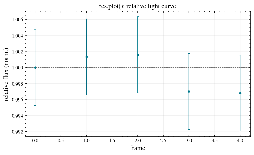
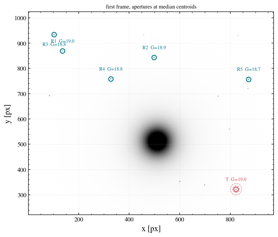
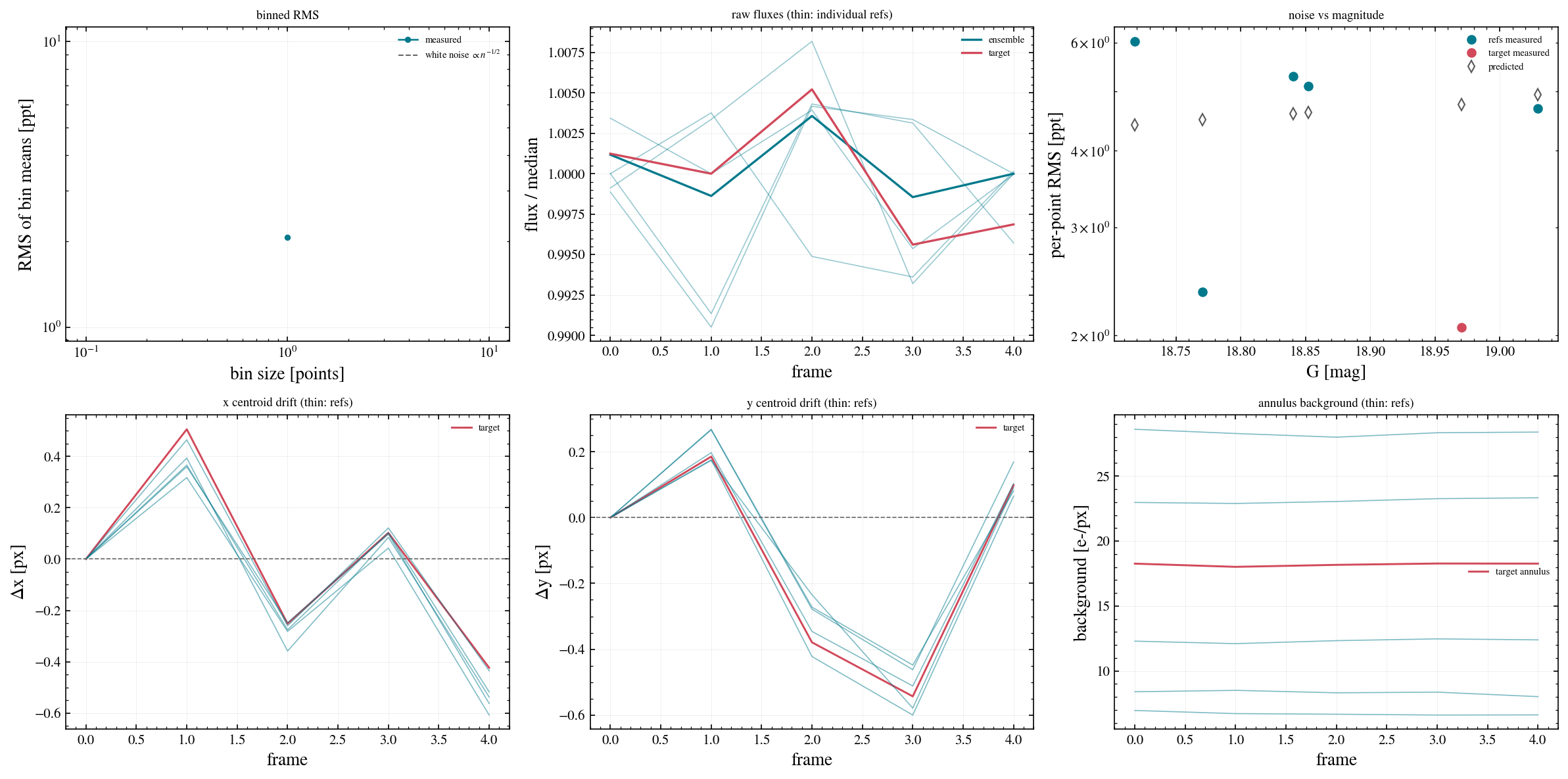
Five dithered frames of the same field, then differential photometry of one of the faint stars against the others. result.plot() is the light curve; plot_field(frame) shows the apertures; the remaining methods are the panels of the diagnostic report, drawn here into one grid through ax=.

from wcc_phot import run_photometry

PIX_DEG = geom.plate_scale_mas / 1000.0 / 3600.0
frames = [field] + [
    simulate_field(RA0 + dx * PIX_DEG, DEC0 + dy * PIX_DEG, sensorfilter='zwo:r', focus=0,
                   exptime=EXPTIME, seed=2 + k, catalog=cat, shape=SHAPE)
    for k, (dx, dy) in enumerate([(0.4, -0.2), (-0.3, 0.3), (0.1, 0.5), (-0.5, -0.1)])
]
faint = field.catalog[~np.asarray(field.catalog['saturated'], dtype=bool)]
target_id = int(faint['source_id'][np.argmin(np.abs(faint['phot_g_mean_mag'] - 19.0))])
res = run_photometry(frames, target=target_id, method='aperture', n_ref=5)
print(f"target {target_id} (G = {res.stars['gmag'][0]:.2f}), {res.params['n_ref']} references, "
      f"r_ap = {res.params['r_ap']:.0f} px")

target 7 (G = 18.97), 5 references, r_ap = 9 px

ax = res.plot()
ax.set_title('res.plot(): relative light curve');

res.plot_field(frames[0]);

fig, axes = plt.subplots(2, 3, figsize=(16, 8))
res.plot_binned_rms(ax=axes[0, 0])
res.plot_raw_fluxes(ax=axes[0, 1])
res.plot_rms_vs_mag(ax=axes[0, 2])
res.plot_centroids(ax=axes[1, 0], coord='x')
res.plot_centroids(ax=axes[1, 1], coord='y')
res.plot_background(ax=axes[1, 2])
plt.tight_layout()

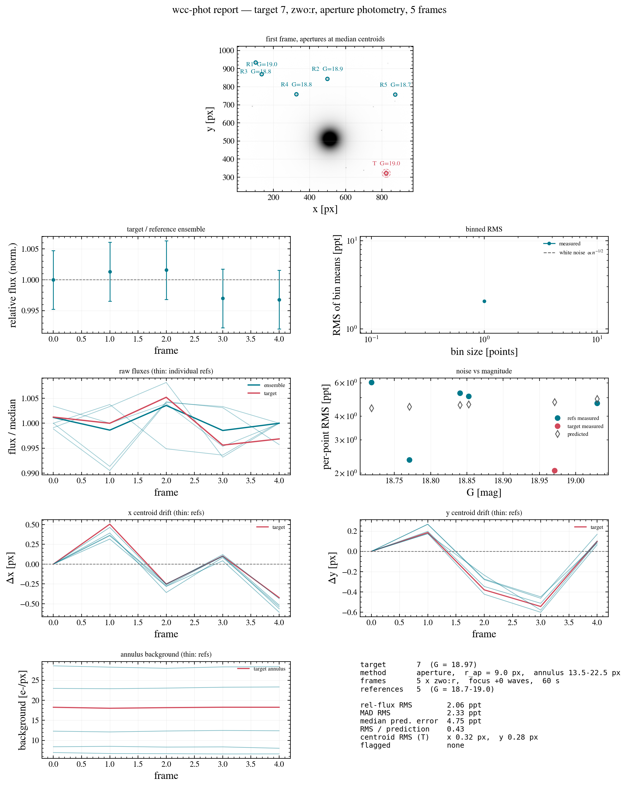
res.report(path, frame=...) writes the same panels, plus a summary block, as a one-page PDF and PNG (the --report flag of wcc-phot does the same from the shell).

paths = res.report(os.path.join(outdir, 'phot_report.pdf'), frame=frames[0])
print('wrote', [os.path.basename(p) for p in paths])

from IPython.display import Image
Image(paths[1], width=700)

wrote ['phot_report.pdf', 'phot_report.png']

Summary

Object	Method	Shows
SimulatedField	plot(which, catalog, satmask)	the image with an asinh stretch
	plot_cutout(star, half_width, which)	a log-stretched cutout around one star
	plot_psf_profile(star)	Airy core, scatter halo, total, and the rendered profile
	plot_satmask()	the saturation mask
	psf_report(path)	the one-page PSF report (PDF + PNG)
PhotometryResult	plot() / plot_lightcurve()	the relative light curve
	plot_field(frame)	the frame with apertures at the median centroids
	plot_binned_rms(), plot_raw_fluxes(), plot_rms_vs_mag()	noise diagnostics
	plot_centroids(coord), plot_background()	per-frame drift and annulus background
	report(path, frame)	the one-page photometry report (PDF + PNG)
wcc_sim.plotting	plot_image, plot_stamp, plot_radial_profile, plot_encircled_energy	the same plots for plain arrays

All of them take ax=None and return the axes. use_style() applies the packaged style to a whole session; without it, only the figures the methods create themselves are styled.