Note

This page is generated from the Jupyter notebook notebooks/08_psf_wings.ipynb in the repository. You can download it and run it interactively.

PSF wings: no more postage stamps

The PSF stamps are finite (129 px in focus, 257 px defocused), so without correction the wing of every bright star is cut to exactly zero at a square boundary. At a hard display stretch that square sits far above the noise, about 100 sigma for a G=8 star in focus at 90 s, which is the classic “postage stamp” artifact in FITS viewers.

With wing extension (wings=True, the default), each star’s stamp is continued beyond its edge with an analytic power-law wing fit from the stamp’s own outer annulus (wcc_sim.wings), on a circular footprint, down to 0.1 sigma of the sky+read noise floor. This notebook verifies the behaviour and quantifies what the wings do to the encircled energy (EE).

The wings fitted here describe the diffraction halo only. The measured scattered-light halo is a separate additive term (scatter=True, also the default, see wcc_sim.scatter and the user guide); field.plot_psf_profile() in notebook 10 shows both terms on one radial profile.

import numpy as np
import matplotlib.pyplot as plt
from astropy.visualization import simple_norm

import wcc_sim
from wcc_sim import simulate_field
from wcc_sim.detectors import make_base_simulation
from wcc_sim.psf import DEFAULT_STAMP, render_oversampled_psf
from wcc_sim.render import bin_oversampled, render_scene
from wcc_sim.wings import fit_wing_model

from wcc_sim.plotting import use_style, TEAL, RED, AMBER, BLUE, plot_radial_profile, encircled_energy
use_style()
print('wcc_sim', wcc_sim.__version__)

wcc_sim 0.1.0

1. Before / after on a real field

A 1024×1024 subarray centered on a G=8.1 star (Gaia DR3 3836000669773723520, near the COSMOS field), simulated with and without wings (same seed, same noise realization). The stretch is set just above the sky to mimic cranking the contrast in a FITS viewer.

RA, DEC = 150.63121, 1.82361  # G = 8.1 star
kw = dict(sensorfilter='zwo:r', focus=0, exptime=90.0, seed=7,
          shape=(1024, 1024), cache_dir='gaia_cache')
field_off = simulate_field(RA, DEC, wings=False, **kw)
field_on = simulate_field(RA, DEC, wings=True, **kw)
star = field_on.catalog[np.argmin(field_on.catalog['phot_g_mean_mag'])]
x0, y0 = int(round(star['x'])), int(round(star['y']))
print(f"G = {star['phot_g_mean_mag']:.2f} at (x, y) = ({x0}, {y0})")
print('wing model: alpha = %.3f, c = %.4f, floor = %.3f e-/pix' % (
    field_on.params['wing_alpha'], field_on.params['wing_c'],
    field_on.params['wing_floor_e']))

G = 8.14 at (x, y) = (510, 511)
wing model: alpha = -2.996, c = 0.0766, floor = 0.328 e-/pix

med = np.median(field_off.image_adu)
norm = simple_norm(field_off.image_adu, 'asinh', vmin=med - 1, vmax=med + 25)
fig, axes = plt.subplots(1, 2, figsize=(11, 5.4), constrained_layout=True)
for ax, f, title in [(axes[0], field_off, 'wings=False (129 px stamp only)'),
                     (axes[1], field_on, 'wings=True (default)')]:
    f.plot(ax=ax, norm=norm, cmap='gray')
    ax.set_title(title)
fig.suptitle('G=8.1 star, SCI [ADU], hard asinh stretch', y=1.04);

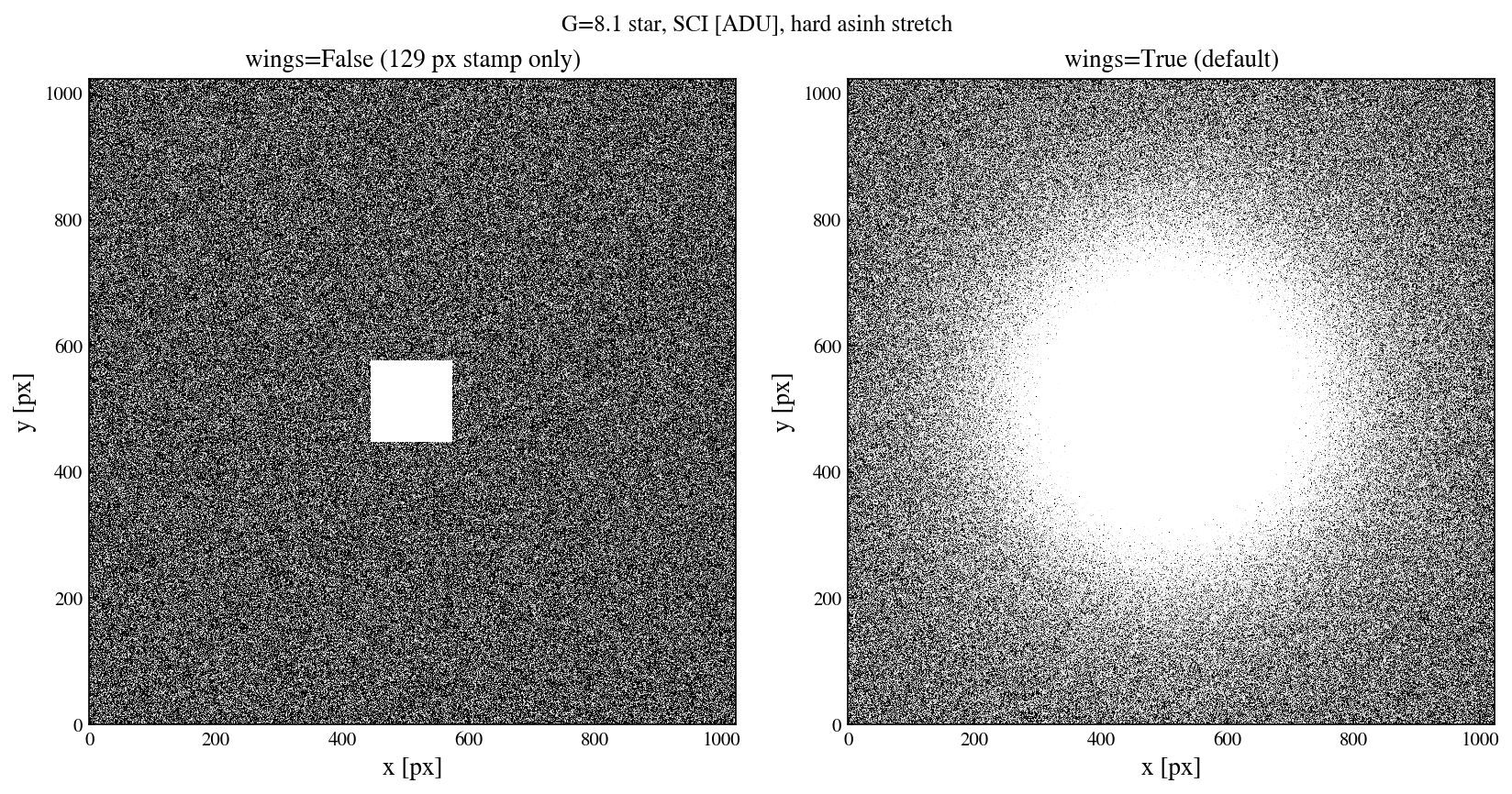
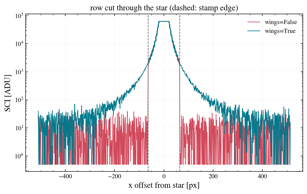
The square is the old stamp boundary; with wings the halo is circular and fades into the noise. A row cut through the star shows the same thing quantitatively: the truncated profile falls off a cliff at ±64 px, the extended one follows the r^-3 Airy envelope down to the noise.

xs = np.arange(1024) - x0
fig, ax = plt.subplots(figsize=(8, 4.6))
ax.semilogy(xs, np.maximum(field_off.image_adu[y0], 0.5), lw=1,
            color=RED, label='wings=False')
ax.semilogy(xs, np.maximum(field_on.image_adu[y0], 0.5), lw=1,
            color=TEAL, label='wings=True')
for edge in (-64, 64):
    ax.axvline(edge, color='0.4', ls='--', lw=1)
ax.set_xlabel('x offset from star [px]'); ax.set_ylabel('SCI [ADU]')
ax.set_title('row cut through the star (dashed: stamp edge)')
ax.legend();

2. The wing model

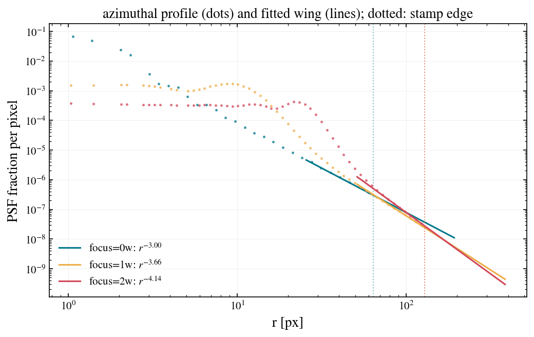
fit_wing_model fits profile(r) = c * r**alpha (PSF fraction per pixel) to the azimuthally smooth outer annulus of the detector-binned stamp. In focus the slope comes out at the physical Airy-envelope value of -3; the defocused Huygens PSFs fall faster. The dots are plot_radial_profile() of each stamp on log-spaced annuli.

sim = make_base_simulation('zwo:r')
wings, stamps = {}, {}
for focus in (0, 1, 2):
    psf_os = render_oversampled_psf(sim, focus, oversample=11)
    stamps[focus] = bin_oversampled(psf_os, 11)
    wings[focus] = fit_wing_model(stamps[focus])
    n = stamps[focus].shape[0]
    print(f'focus={focus}w  stamp={n:3d} px  '
          f'alpha={wings[focus].alpha:6.2f}  c={wings[focus].c:.3e}')

focus=0w  stamp=129 px  alpha= -3.00  c=7.663e-02

/Users/gudmundurstefansson/Dropbox/mypylib/notebooks/GIT/wcc-sim/src/wcc_sim/psf.py:35: RuntimeWarning: divide by zero encountered in matmul
  cx = (psf.sum(axis=0) @ i) / total
/Users/gudmundurstefansson/Dropbox/mypylib/notebooks/GIT/wcc-sim/src/wcc_sim/psf.py:35: RuntimeWarning: overflow encountered in matmul
  cx = (psf.sum(axis=0) @ i) / total
/Users/gudmundurstefansson/Dropbox/mypylib/notebooks/GIT/wcc-sim/src/wcc_sim/psf.py:35: RuntimeWarning: invalid value encountered in matmul
  cx = (psf.sum(axis=0) @ i) / total
/Users/gudmundurstefansson/Dropbox/mypylib/notebooks/GIT/wcc-sim/src/wcc_sim/psf.py:36: RuntimeWarning: divide by zero encountered in matmul
  cy = (psf.sum(axis=1) @ i) / total
/Users/gudmundurstefansson/Dropbox/mypylib/notebooks/GIT/wcc-sim/src/wcc_sim/psf.py:36: RuntimeWarning: overflow encountered in matmul
  cy = (psf.sum(axis=1) @ i) / total
/Users/gudmundurstefansson/Dropbox/mypylib/notebooks/GIT/wcc-sim/src/wcc_sim/psf.py:36: RuntimeWarning: invalid value encountered in matmul
  cy = (psf.sum(axis=1) @ i) / total

focus=1w  stamp=257 px  alpha= -3.66  c=1.261e+00
focus=2w  stamp=257 px  alpha= -4.14  c=1.518e+01

fig, ax = plt.subplots(figsize=(8, 4.6))
colors = {0: TEAL, 1: AMBER, 2: RED}
for focus in (0, 1, 2):
    stamp, w = stamps[focus], wings[focus]
    half = stamp.shape[0] // 2
    plot_radial_profile(stamp, half, half, ax=ax, r_max=half, n_bins=half // 2, log=True,
                        marker='.', ls='none', ms=3, color=colors[focus], alpha=0.6)
    rr = np.linspace(0.4 * half, 3 * half, 100)
    ax.loglog(rr, w.profile(rr), '-', color=colors[focus], lw=1.5,
              label=f'focus={focus}w: $r^{{{w.alpha:.2f}}}$')
    ax.axvline(half, color=colors[focus], ls=':', lw=1, alpha=0.5)
ax.set_xlabel('r [px]'); ax.set_ylabel('PSF fraction per pixel')
ax.set_title('azimuthal profile (dots) and fitted wing (lines); dotted: stamp edge')
ax.legend();

3. Seam smoothness

The fix has two parts: the stamp’s outer 20% is crossfaded into the smooth model (so Airy-ring texture doesn’t stop abruptly), and the halo continues outside on a circular footprint. On the noiseless image the profile should now cross the old stamp edge without any visible jump.

half = 64  # 129 px in-focus stamp
row_off = field_off.image_clean[y0]
row_on = field_on.image_clean[y0]
jump_off = abs(row_off[x0 + half] - row_off[x0 + half + 2])
jump_on = abs(row_on[x0 + half] - row_on[x0 + half + 2])
local = row_on[x0 + half]
print(f'clean-image step across the stamp edge, wings off: {jump_off:9.1f} e-')
print(f'clean-image step across the stamp edge, wings on : {jump_on:9.1f} e-')
print(f'local wing level there: {local:.1f} e-/pix '
      f'-> relative jump {jump_on / local:.1%}')
assert jump_on / local < 0.15, 'seam should be smooth'
assert jump_off / local > 0.5, 'truncated case should be a cliff'

clean-image step across the stamp edge, wings off:     525.2 e-
clean-image step across the stamp edge, wings on :      47.1 e-
local wing level there: 541.1 e-/pix -> relative jump 8.7%

4. Encircled energy: what do the wings change?

Two effects, both small and physical:

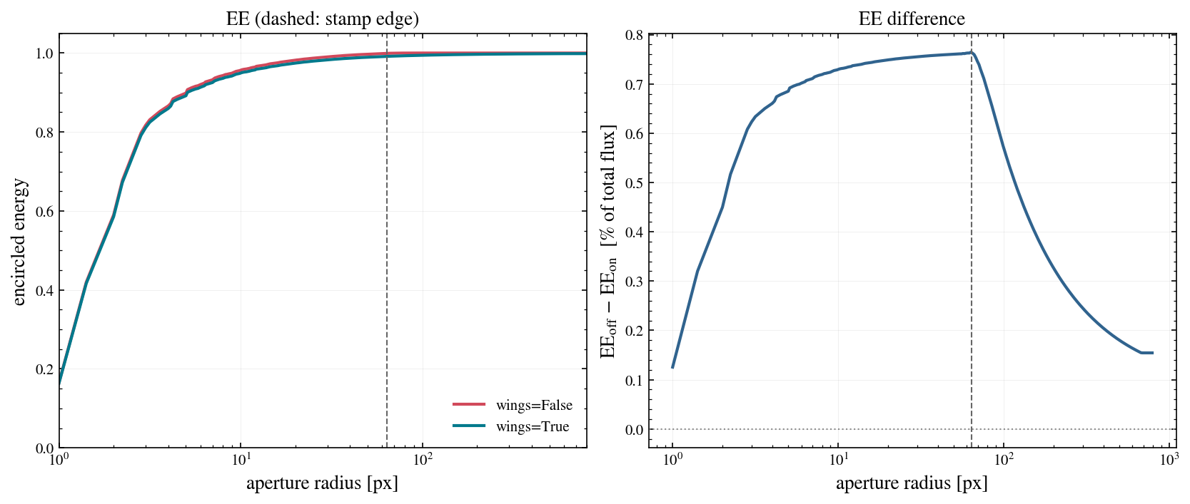
1. Renormalization. The truncated stamp pretended 100% of the flux landed inside the stamp. With wings, every star is scaled by 1/(1 + E_wing) where E_wing is the wing energy beyond the stamp edge, so EE inside any small aperture drops by that fraction.

2. The halo itself. EE keeps growing beyond the old stamp edge instead of flat-lining at 1.0.

Below: EE curves for a single in-focus star rendered noiselessly with and without wings (flux 10⁹ e⁻, halo drawn to its 0.25 e⁻/pix floor at ~680 px).

N = 1601; c0 = N // 2; flux = 1e9
psf0 = render_oversampled_psf(sim, 0, oversample=11)
img_ee_off = render_scene((N, N), [c0], [c0], [flux], psf0, 11)
img_ee_on = render_scene((N, N), [c0], [c0], [flux], psf0, 11,
                         wing=wings[0], floor_e=0.25)
# normalised to the star's true flux, not the image sum, so a truncated render shows up as EE < 1
r_sorted, ee_off = encircled_energy(img_ee_off, total=flux)
_, ee_on = encircled_energy(img_ee_on, total=flux)
E_wing = wings[0].energy_beyond(64.0)
print(f'total flux ratio, wings on : {img_ee_on.sum() / flux:.4f}')
print(f'total flux ratio, wings off: {img_ee_off.sum() / flux:.4f}')
print(f'analytic wing energy beyond the 129 px stamp: {E_wing:.4f} '
      f'({E_wing / (1 + E_wing):.2%} of total flux)')
assert abs(img_ee_on.sum() / flux - 1.0) < 0.01

total flux ratio, wings on : 0.9985
total flux ratio, wings off: 1.0000
analytic wing energy beyond the 129 px stamp: 0.0077 (0.76% of total flux)

idx = np.unique(np.searchsorted(r_sorted, np.logspace(0, np.log10(790), 300)))
fig, (ax1, ax2) = plt.subplots(1, 2, figsize=(11, 4.6), constrained_layout=True)
ax1.semilogx(r_sorted[idx], ee_off[idx], color=RED, label='wings=False')
ax1.semilogx(r_sorted[idx], ee_on[idx], color=TEAL, label='wings=True')
ax1.axvline(64, color='0.4', ls='--', lw=1)
ax1.set_xlabel('aperture radius [px]'); ax1.set_ylabel('encircled energy')
ax1.set_xlim(1, 800); ax1.set_ylim(0, 1.05)
ax1.set_title('EE (dashed: stamp edge)')
ax1.legend(loc='lower right')

ax2.semilogx(r_sorted[idx], (ee_off - ee_on)[idx] * 100, color=BLUE)
ax2.axvline(64, color='0.4', ls='--', lw=1)
ax2.axhline(0, color='0.55', ls=':', lw=1)
ax2.set_xlabel('aperture radius [px]')
ax2.set_ylabel(r'EE$_{\rm off}$ $-$ EE$_{\rm on}$  [% of total flux]')
ax2.set_title('EE difference');

radii = [2, 5, 10, 20, 40, 64, 100, 200, 400, 680]
print(' r [px]   EE off    EE on    diff [%]')
for rad in radii:
    i = np.searchsorted(r_sorted, rad)
    print(f'{rad:6d}   {ee_off[i]:.4f}   {ee_on[i]:.4f}   '
          f'{(ee_off[i] - ee_on[i]) * 100:+7.3f}')
assert np.all(np.diff(ee_on[::997]) > -1e-9), 'EE must be monotonic'

 r [px]   EE off    EE on    diff [%]
     2   0.5900   0.5855    +0.450
     5   0.8986   0.8917    +0.685
    10   0.9564   0.9491    +0.729
    20   0.9820   0.9745    +0.749
    40   0.9945   0.9869    +0.758
    64   0.9992   0.9916    +0.765
   100   1.0000   0.9943    +0.571
   200   1.0000   0.9967    +0.327
   400   1.0000   0.9980    +0.205
   680   1.0000   0.9985    +0.154

Inside the core the EE simply drops by the renormalization factor, a uniform ≈0.7% for the in-focus 129 px stamp. Beyond the stamp edge the wings return that energy, closing back to 100% at the halo’s truncation radius.

The same number per focus mode, from the fitted models (this is the total flux each mode’s default stamp used to overcount):

print('focus  stamp   alpha   flux beyond stamp')
for focus in (0, 1, 2):
    w = wings[focus]
    half_f = DEFAULT_STAMP[focus] // 2
    E = w.energy_beyond(half_f)
    print(f'{focus:3d}w   {DEFAULT_STAMP[focus]:4d}px  {w.alpha:6.2f}   '
          f'{E / (1 + E):.3%}')

focus  stamp   alpha   flux beyond stamp
  0w    129px   -3.00   0.763%
  1w    257px   -3.66   0.152%
  2w    257px   -4.14   0.135%

5. How far do the wings extend in practice?

The halo is drawn out to r_out, where flux * profile(r) drops to the 0.1 sigma floor; with an r^-3 wing that radius scales as flux^(1/3). Against the full IMX455 frame:

from astropy.table import Table
from wcc_sim.detectors import get_geometry
from wcc_sim.starflux import rates_for_catalog

geom = get_geometry('zwo:r', sim=sim)
print(f'detector: {geom.nx} x {geom.ny} px '
      f'(diagonal {np.hypot(geom.nx, geom.ny):.0f} px), '
      f'{geom.plate_scale_mas:.2f} mas/px')

mags = np.arange(0.0, 15.0, 2.0)
cat = Table({'phot_g_mean_mag': mags,
             'phot_bp_mean_mag': mags + 0.4,
             'phot_rp_mean_mag': mags - 0.4,
             'ra': np.zeros_like(mags), 'dec': np.zeros_like(mags)})
rates, _ = rates_for_catalog(cat, 'zwo:r')
exptime, floor = 90.0, field_on.params['wing_floor_e']
well = sim.sensor.meta['well_depth']
print(f'\n  G    flux (90 s)    r_out 0w [px]  [arcsec]   r_out 2w   sat-halo 0w')
for G, rate in zip(mags, rates):
    f = rate * exptime
    r0, r2 = wings[0].r_out(f, floor), wings[2].r_out(f, floor)
    rsat = (wings[0].c * f / well) ** (-1 / wings[0].alpha) \
        if wings[0].c * f > well else 0.0
    print(f'{G:4.0f}   {f:10.2e}   {r0:10.0f}   {r0 * geom.plate_scale_mas / 1e3:8.1f}'
          f'   {r2:8.0f}   {rsat:8.0f} px')

detector: 9568 x 6380 px (diagonal 11500 px), 16.87 mas/px

  G    flux (90 s)    r_out 0w [px]  [arcsec]   r_out 2w   sat-halo 0w
   0     3.43e+12         9405      158.7       2670        255 px
   2     5.44e+11         5085       85.8       1712        138 px
   4     8.62e+10         2750       46.4       1098         74 px
   6     1.37e+10         1487       25.1        704         40 px
   8     2.17e+09          804       13.6        451         22 px
  10     3.43e+08          435        7.3        289         12 px
  12     5.44e+07          235        4.0        185          6 px
  14     8.62e+06          127        2.1        128          3 px

A 0-mag star’s wing reaches ~9,400 px (~160 arcsec), essentially the whole detector, and that is physically correct: at 3,000 px its diffraction wing is still ~10 e⁻/pix ≈ 3 sigma above sky, a real detectable gradient across the frame. The drawn halo always ends at 0.1 sigma, so the outer cutoff stays invisible. The brightest stars also saturate a large disk (~255 px radius for G=0, the “sat-halo” column). Full-frame halos are evaluated in row chunks, so even a G=0 star costs only a few seconds.

6. Is the extrapolation correct?

Two independent arguments for the in-focus PSF:

1. The physics fixes the law. r^-3 is the exact asymptotic envelope of the circular-aperture Airy pattern; the fit recovering alpha = -2.996 means the stamp’s outer annulus is already in that regime. Jitter and broadband smearing smooth the rings but do not change the envelope.

2. Direct test against the physical-optics code. Below we render the wcc_etc PSF at 1025 px (8x the production stamp) and compare its measured profile with the power law extrapolated from the 129 px fit.

psf_big = render_oversampled_psf(sim, 0, oversample=1, stamp_npix=1025)
nb_ = psf_big.shape[0]; hb = nb_ // 2
yy, xx = np.mgrid[:nb_, :nb_]
rbig = np.hypot(yy - hb, xx - hb)
radii_chk = [80, 120, 180, 260, 360, 480]
print(' r [px]   rendered PSF   c*r^alpha    ratio')
ratios = []
for r0 in radii_chk:
    m = (rbig > r0 - 2) & (rbig < r0 + 2)
    meas = np.median(psf_big[m])
    model = wings[0].profile(r0)
    ratios.append(meas / model)
    print(f'{r0:6d}   {meas:.3e}   {model:.3e}   {meas / model:6.2f}')
assert max(abs(np.log(ratios))) < np.log(1.2), \
    'extrapolation should match physical optics to <20%'

 r [px]   rendered PSF   c*r^alpha    ratio
    80   1.439e-07   1.524e-07     0.94
   120   4.444e-08   4.523e-08     0.98
   180   1.372e-08   1.342e-08     1.02
   260   4.788e-09   4.461e-09     1.07
   360   1.660e-09   1.683e-09     0.99
   480   6.907e-10   7.107e-10     0.97

fig, ax = plt.subplots(figsize=(8, 4.6))
plot_radial_profile(psf_big, hb, hb, ax=ax, r_max=hb - 2, n_bins=60, log=True,
                    marker='.', ls='none', ms=4, color=BLUE,
                    label='physical-optics render (1025 px)')
rr = np.geomspace(25, hb, 100)
ax.loglog(rr, wings[0].profile(rr), '-', color=TEAL, lw=1.5,
          label=f'wing fit from 129 px stamp: $r^{{{wings[0].alpha:.2f}}}$')
ax.axvspan(0.65 * 64, 0.98 * 64, color=AMBER, alpha=0.2,
           label='fit annulus (129 px stamp)')
ax.axvline(64, color='0.4', ls='--', lw=1)
ax.set_xlabel('r [px]'); ax.set_ylabel('PSF fraction per pixel')
ax.set_title('extrapolation check: agrees to $\\pm$7% out to 480 px')
ax.legend();

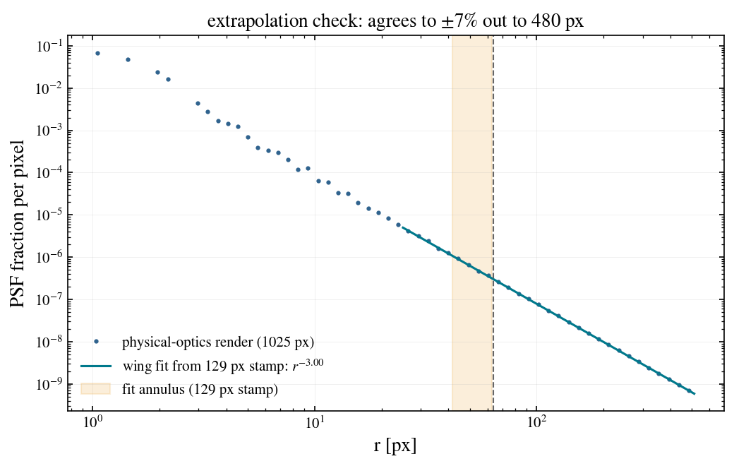
For the defocused PSFs the fitted slopes (-3.7, -4.2) are only backed by the Huygens data out to its ~272 px span; far enough out the wing should revert to the r^-3 diffraction envelope, so the defocused far wings are likely slight underestimates beyond a few hundred px (small in absolute terms, since their wing amplitudes are about 10x lower to begin with).

For the brightest stars the far halo at arcminute scales is dominated by scattered light (mirror micro-roughness, particulates), which is shallower (about r^-2) and brighter than pure diffraction. That term is modelled separately from the FRED stray-light ray trace and added on top of these wings (scatter=True); the diffraction wings alone are a lower bound on the far halo.

Summary

• Truncated stamps put a square, ~100-sigma cliff around every bright star; with wings=True the halo is circular, follows the fitted power law, and ends below 0.1 sigma of the noise floor.

• The seam at the old stamp edge is smooth (relative jump at the percent level, on a signal that is itself deep in the wing).

• Encircled energy changes by the wing renormalisation: about 0.7% less flux in any core aperture for the in-focus 129 px stamp (about 0.1% for the defocused 257 px stamps), returned in the halo so the total closes to 100% within 1%.

• Photometry stays magnitude independent: every star gets the same renormalisation whether or not its (sub-noise) halo is drawn.

• Wing extent scales as flux^(1/3): about 4 arcsec at G=12, the full detector at G=0, which is physically expected for a 0-mag star.

• The in-focus extrapolation matches an 8x larger physical-optics render to +/-7% (and r^-3 is the analytic Airy envelope); the defocused slopes are an assumption beyond the ~272 px Huygens data span.

• The scattered-light halo is a separate, additive term of the PSF; see the scattered-light page of the user guide and field.plot_psf_profile().