Note

This page is generated from the Jupyter notebook notebooks/01_getting_started.ipynb in the repository. You can download it and run it interactively.

01 Getting started with esc_etc

esc_etc is the exposure-time calculator for the ESC, the coronagraphic camera on Lazuli, a 3 m telescope. It answers two questions: what signal-to-noise ratio (SNR) a planet reaches in a given integration time, and how long it takes to reach a target SNR. This notebook goes from an empty session to both answers, then shows where the noise comes from.

Requirements: pip install -e . from the repo root. The instrument configuration (UM 3 m ESC) ships inside the package, so nothing else needs to be installed.

import astropy.units as u
import esc_etc
from esc_etc import Simulation, use_lazuli_style

use_lazuli_style()      # house plotting style for the whole session
print('esc_etc', esc_etc.__version__)

esc_etc 0.1.0.post31+ge8d3be707.d20261010

1. A default simulation

Simulation.from_default() builds the four pieces of the calculator (telescope, sensor, scene, coronagraph) from the packaged configuration. The arguments below are the defaults, written out so you can see what a scene is: a host star of Vega magnitude -0.353, a planet 20 magnitudes fainter at 0.2 arcsec, a raw dark-hole contrast of 1e-8, and a post-processing gain of 10. The bandpass is the end-of-life curve of the F630N filter (notebook 02 shows the alternatives). Magnitudes are quoted in the ESC band unless you say otherwise (notebook 02).

sim = Simulation.from_default(
    hoststarmag=-0.353, planetdeltamag=20,
    contrast=1e-8, ppgain=10, separation=0.2,
)
sim

<esc_etc.simulation.Simulation at 0x1332dacf0>

2. SNR for a given integration time

get_snr takes the total on-target time and the length of one detector frame. Both accept astropy quantities or plain numbers, which are read as seconds. The result is a dictionary: snr, the integrated planet signal and total noise in electrons, and M, the post-processing noise floor (more on that in notebook 03).

out = sim.get_snr(total_time=3600 * u.s, frame_time=100 * u.s)
print('SNR          :', round(out['snr'], 3))
print('signal [e-]  :', round(out['signal_e'], 1))
print('noise  [e-]  :', round(out['noise_e'], 1))

# plain floats are seconds; hours work too
assert sim.get_snr(3600, 100)['snr'] == out['snr']
assert sim.get_snr(1 * u.h, 100)['snr'] == out['snr']
assert abs(out['snr'] - 9.75) < 0.05, out['snr']

SNR          : 9.747
signal [e-]  : 4811.8
noise  [e-]  : 493.7

3. Integration time for a target SNR

get_int_time_for_snr is the inverse. int_time is rounded up to whole frames; int_time_continuous is the exact solution. The 3600 s above round-trips. SNR 5 is reached in about 30 s because it is only half of this scene’s plateau of 10; the last factor of two toward the plateau takes most of the hour (notebook 03 explains the plateau).

back = sim.get_int_time_for_snr(out['snr'], frame_time=100)
five = sim.get_int_time_for_snr(5, frame_time=100)
print('time to recover the SNR above :', back['int_time'][0])
print('time to SNR 5                 :', five['int_time_continuous'][0])
assert abs(back['int_time'][0].value - 3600) < 1

time to recover the SNR above : 3600.0 s
time to SNR 5                 : 63.160285873583575 s

4. Where the noise comes from

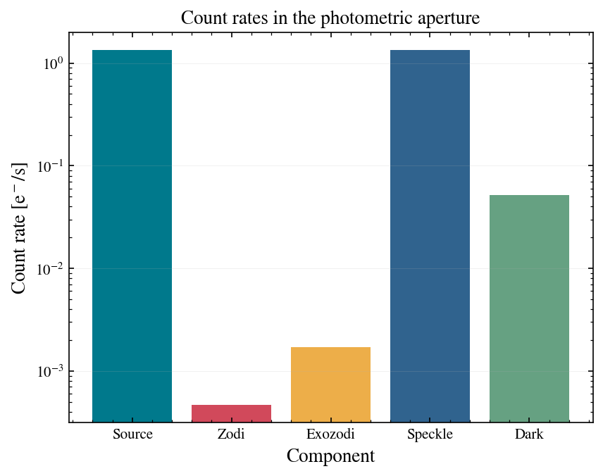
count_rate_components returns the per-second electron rates inside the photometric aperture: the planet (source), zodiacal and exozodiacal light, residual speckles, and the host rate after the focal-plane mask. The speckle rate is host x contrast x EE, where EE is the fraction of a point source that falls inside the aperture (0.456 for the default aperture, see notebook 02): 5.4e8 x 1e-8 x 0.456 = 2.48 e/s. The planet gets the same EE factor, so with a contrast of 1e-8 and a planet 20 mag fainter the two rates come out equal, which is no accident: 10^(-0.4 x 20) = 1e-8.

rates = sim.count_rate_components()
for name in ['source', 'zodi', 'exozodi', 'speckle', 'host']:
    print(f'{name:8s}: {getattr(rates, name):.3e}')

fig, ax = sim.plot_count_rates()
ax.set_title('Count rates in the photometric aperture');

source  : 1.337e+00 electron / s
zodi    : 4.659e-04 electron / s
exozodi : 1.720e-03 electron / s
speckle : 1.337e+00 electron / s
host    : 2.932e+08 electron / s

5. Everything at once

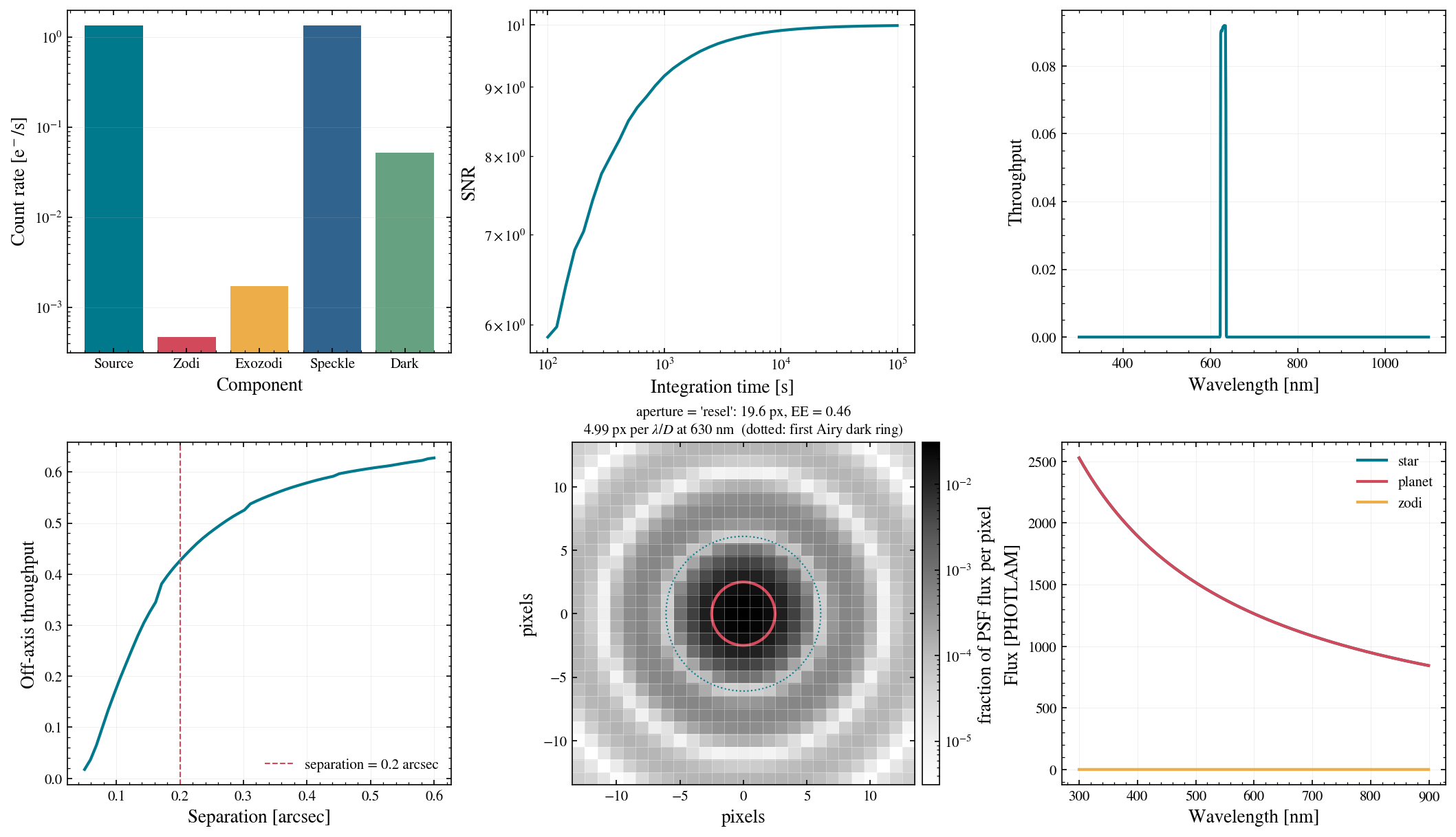
sim.plot() draws the six standard panels. Every panel is also its own method (sim.plot_snr_vs_time(), sim.plot_bandpass(), and so on), and each accepts ax= so you can place it in your own figure.

fig, axes = sim.plot()

Notebook 02 takes the simulation apart into its components and shows how to change parameters.