Saturation

esc-etc reports saturation as a frame time: the longest single frame you can read out before the brightest pixel in the planet’s aperture fills the well. The noise model reads an integration out in frames of duration frame_time (see Signal-to-noise and integration time), so saturation limits that frame time. The total integration can be as long as you like.

The saturation time

saturation_time() divides the usable well by the peak-pixel electron rate:

\[t_\mathrm{sat} = \frac{h\,W}{f_\mathrm{peak}\left(R_\mathrm{source} + R_\mathrm{speckle}\right) + \left(R_\mathrm{zodi} + R_\mathrm{exozodi}\right) / N_\mathrm{pix} + R_\mathrm{dark}}\]

where \(W\) is Sensor.well_depth, \(h\) is Sensor.headroom (the usable fraction of the full well, default 0.8), \(f_\mathrm{peak}\) is Sensor.peak_pixel_fraction (the share of a point source’s in-aperture rate that lands on its brightest pixel), \(N_\mathrm{pix}\) is Sensor.num_psf_pixels and \(R_\mathrm{dark}\) is the dark current per pixel. The planet and the speckles are point-like, so their light concentrates on one pixel; the backgrounds are uniform, so each pixel gets an equal share. The rates come from count_rate_components():

sim.saturation_time()         # seconds
sim.is_saturated(100)         # True / False for a 100 s frame

is_saturated() is the comparison frame_time > saturation_time(), so both use the same definition.

Note

The occulted host star is not modelled. The pixel in question is the brightest one in the planet’s aperture, where starlight has been suppressed to the raw contrast, not the stellar core behind the focal-plane mask or the bright ring just inside the dark hole. For a bright host those pixels saturate much sooner, so treat this frame time as an upper bound (see Known limitations). All rates already include the mask throughput coronagraph.off_axis_throughput.

What sets the peak-pixel rate

Three sensor parameters move \(t_\mathrm{sat}\) for a fixed scene, all mutable through Simulation.update.

well_depth is read from the detector table for the configured gain setting, and headroom is a safety margin on it rather than a measured linearity limit:

sim.update(sensor__well_depth=60000, sensor__headroom=0.9)   # electrons per pixel
sim.saturation_time()
sim.reset()

peak_pixel_fraction defaults to the value for an Airy pattern at the sensor plate scale. The peak surface brightness of an Airy pattern is \(\pi/4\) of the total flux per \((\lambda/D)^2\); dividing by the pixel area and by the encircled energy inside the aperture gives the share of the in-aperture rate on the brightest pixel. At the default configuration this is about 0.069, against 0.051 for the aperture mean. It ignores Lyot-stop broadening, pointing jitter and the integration over a finite pixel. When a real PSF image is available, set the fraction from it:

# psf_image: a 2-D array of the planet PSF sampled at the detector plate scale
sim.update(sensor__peak_pixel_fraction=psf_image.max() / psf_image.sum())

Choosing a frame time

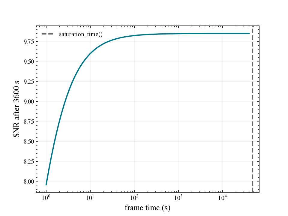
Saturation pushes frame_time down; read noise pushes it up. The read-noise term in the noise budget is \(\sigma_\mathrm{read}^2 \, N_\mathrm{pix} \, N_\mathrm{reads}\) with \(N_\mathrm{reads} = \lceil t_\mathrm{total} / t_\mathrm{frame} \rceil\), so splitting a long integration into many short frames to avoid saturation costs SNR.

Because headroom already holds back part of the well, a frame time at or just under \(t_\mathrm{sat}\) is the natural choice:

frame_time = sim.saturation_time()
result = sim.get_snr(total_time=3600, frame_time=frame_time)

The trade-off for the default scene, with the saturation time marked. Once the frame is longer than the whole integration there is a single read, so the curve is flat beyond one hour:

import numpy as np
import matplotlib.pyplot as plt
from esc_etc import Simulation, lazuli_style

sim = Simulation.from_default(separation=0.4, contrast=1e-8, ppgain=10)
frame_times = np.logspace(0, 4.6, 80)                      # 1 s to 40 000 s
snr = [sim.get_snr(total_time=3600, frame_time=ft)["snr"] for ft in frame_times]

with lazuli_style():
    fig, ax = plt.subplots()
    ax.semilogx(frame_times, snr)
    ax.axvline(sim.saturation_time().value, ls="--", color="0.4", label="saturation_time()")
    ax.set_xlabel("frame time (s)")
    ax.set_ylabel("SNR after 3600 s")
    ax.legend()

Tip

If saturation_time() comes back shorter than a practical readout cadence, shortening the total exposure does not help, since only the individual frame is constrained. What helps is a fainter host, a better contrast or a deeper well.

04 Integration time, frames and saturation sweeps the frame time against both saturation and SNR.