Coronagraph and contrast
The vocabulary
A coronagraph blocks the light of the host star so that a planet next to it can be seen. In the ESC, a vector vortex focal-plane mask sits where the star is imaged and diverts its light; a Lyot stop in the following pupil plane then removes the diffracted starlight, at the cost of a slightly smaller effective aperture and a slightly wider PSF. Some starlight still leaks through, because the wavefront is never perfect, and lands on the detector as a pattern of speckles that looks like a field of faint point sources.
Deformable mirrors correct the wavefront over a region around the star, the dark hole, where the leaked starlight is suppressed to a level called the raw contrast: the residual starlight in a resolution element, relative to the peak of the unocculted star. A raw contrast of \(10^{-8}\) means the speckles in the dark hole are as bright as a planet 20 magnitudes fainter than its host.
Speckles are partly static, so post-processing (subtracting a reference image
or a model of the speckle pattern) can remove a further factor, the
post-processing gain ppgain. What it cannot remove is their photon
noise, which is counted in full, and the part of the pattern that survives
subtraction, which sets a noise floor and hence a maximum signal-to-noise
(see Signal-to-noise and integration time).
Angles in coronagraphy are measured in units of \(\lambda/D\), the diffraction scale. For the ESC at 630 nm on the 3 m aperture, 1 \(\lambda/D\) is 0.043 arcsec, so the default planet separation of 0.4 arcsec is about 9 \(\lambda/D\). A planet close to the mask is partly blocked by it; the off-axis throughput curve gives the fraction that gets through as a function of separation.
Parameters
Parameter |
Meaning |
|---|---|
|
The raw dark-hole contrast, for example |
|
The assumed post-processing gain. It divides the systematic speckle
floor ( |
|
|
|
RDI only: the reference star’s brightness relative to the host, and the reference exposure time relative to the science time. |
|
The planet’s angular separation in arcsec. It selects the off-axis throughput from the mask curve. |
The off-axis throughput
off_axis_throughput() converts a separation in
arcsec to \(\lambda/D\) (using the filter wavelength and the primary
diameter) and looks up the focal-plane mask transmission in the curve loaded
from the instrument configuration. At 0.4 arcsec the throughput is 0.58:
from esc_etc import Simulation

sim = Simulation.from_default(separation=0.4, contrast=1e-8, ppgain=10)
sim.coronagraph.off_axis_throughput()        # at the current separation: 0.58
sim.coronagraph.off_axis_throughput(0.6)     # at 0.6 arcsec
fig, ax = sim.coronagraph.plot_offaxis_throughput()   # the whole curve, separation marked
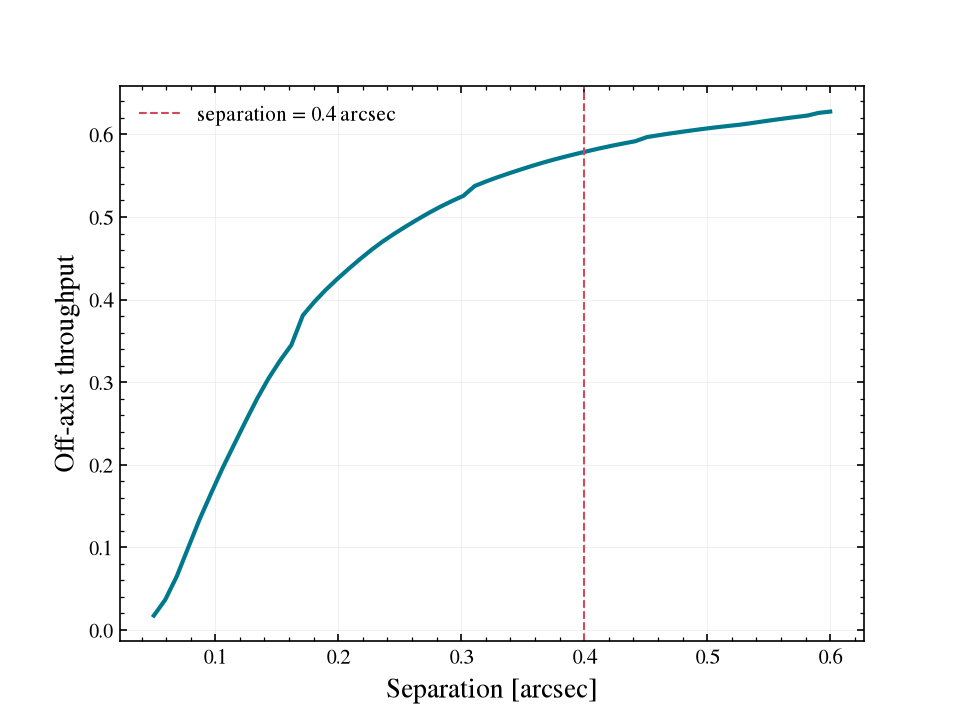
This throughput \(k\) is applied as one scalar to every count rate in
count_rate_components(): planet, speckle, zodi,
exozodi and the reported host rate are all multiplied by it. That is a
simplification; the curve is tabulated at 0.2 \(\lambda/D\) steps and
read with the nearest point, and no inner working angle is enforced, so a
separation well inside the mask returns a small throughput rather than an
error (see Known limitations).
Sweeping the parameters
Update any parameter and recompute. To see how SNR responds to a larger assumed post-processing gain:
for ppg in (5, 10, 20, 50):
    sim.update(coronagraph__ppgain=ppg)
    print(ppg, sim.get_snr(3600, 100)["snr"])

sim.reset()
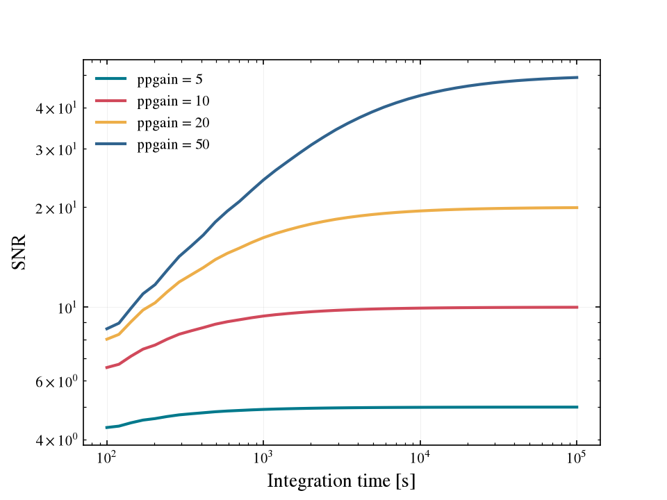
plot_snr_vs_time(sweep=...) draws the same sweep as one curve per value.
Each curve flattens at its own ceiling, ppgain times the planet-to-speckle
ratio (see Signal-to-noise and integration time):
fig, ax = sim.plot_snr_vs_time(sweep={"coronagraph__ppgain": [5, 10, 20, 50]})
See Plotting for the other plot methods.