Note

This page is generated from the Jupyter notebook notebooks/02_components_and_parameters.ipynb in the repository. You can download it and run it interactively.

02 Components and parameters

A Simulation is a Telescope, a Sensor, a Scene and a Coronagraph. This notebook builds each one, looks at what it holds, assembles them by hand, and changes parameters with update() and reset(). It also covers the two choices that most affect the numbers: the photometric aperture and the filter curve.

Requirements: an editable install (pip install -e .), as in notebook 01.

import numpy as np
import astropy.units as u
import matplotlib.pyplot as plt
from esc_etc import (Telescope, Sensor, get_scene, Coronagraph, Simulation,
                     FILTERS, use_lazuli_style)
use_lazuli_style()

1. Telescope

The collecting area is the Lyot-stop area, which is smaller than the 3 m primary. resel is the solid angle of a disk of diameter lambda/D at the design wavelength; it is the default photometric aperture.

t = Telescope.from_default()
print('primary diameter :', t.diameter_primary)
print('collecting area  :', t.surface)
print('f-number         :', round(t.f_num, 1))
print('resel            :', t.resel)

primary diameter : 3.0 m
collecting area  : 5.725552611167399 m2
f-number         : 36.7
resel            : 0.0014735970287905057 arcsec2

2. Sensor: detector and bandpass

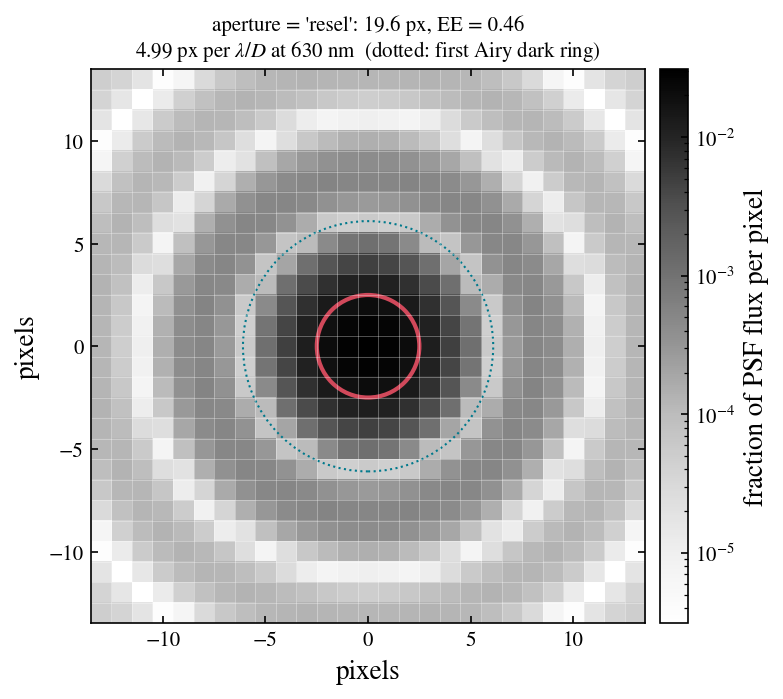
The sensor holds the detector noise properties and the full non-coronagraphic throughput curve (bandpass). num_psf_pixels is the photometric aperture in detector pixels and ee_fraction is the fraction of an unaberrated Airy pattern that lands inside it. Both follow from aperture:

aperture	what it is	pixels	encircled energy
"resel" (default)	disk of diameter lambda/D	19.6	0.46
"optimal"	disk of radius 0.7 lambda/D	38	0.68
"box"	square of side 2.44 lambda/D	169	0.85
"matched"	PSF-weighted sum; the matched-filter limit, not what a pipeline delivers	70 (effective)	1.00

The SNR barely moves between them for this scene because it is speckle limited, so the choice matters more for faint planets where read noise and background count. You can also override encircled_energy directly; it must be a fraction in (0, 1].

s = Sensor.from_default(t)
print('gain         :', s.gain)
print('read noise   :', s.read_noise)
print('dark current :', s.dark_current)
print('well depth   :', s.well_depth)
print('aperture     :', s.aperture, '|', s.num_psf_pixels, '| EE', round(s.ee_fraction, 3))
assert np.isclose(s.num_psf_pixels.value * s.plate_scale**2, t.resel.value)

fig, ax = s.plot_aperture()

gain         : 0.9239970596457494 electron / ct
read noise   : 1.832077426554004 electron(1/2) / pix(1/2)
dark current : 0.0026523364364736 electron / (pix s)
well depth   : 15260.992347242305 electron / pix
aperture     : resel | 19.595181216030333 pix | EE 0.456

3. Filters

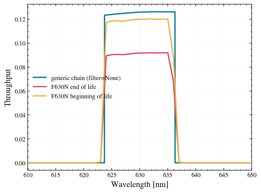
FILTERS lists the ESC filter set. Passing filter= to Simulation.from_default uses that filter’s measured curve as the whole bandpass and moves the telescope’s design wavelength to match; lifetime="eol" (the default) or "bol" selects the end-of-life or beginning-of-life curve. The default is DEFAULT_FILTER (F630N, end of life). filter=None is the legacy option: the generic configuration chain, which is wider and a little more transmissive than any real filter.

When you build the components yourself, the telescope and the sensor must be built for the same filter. Mixing them raises a ValueError, because the pixel geometry would be computed at one wavelength and the throughput at another.

print(sorted(FILTERS))

fig, ax = plt.subplots()
Simulation.from_default(filter=None).plot_bandpass(ax=ax, label='generic chain (filter=None)')
Simulation.from_default(filter='F630N', lifetime='eol').plot_bandpass(ax=ax, label='F630N end of life')
Simulation.from_default(filter='F630N', lifetime='bol').plot_bandpass(ax=ax, label='F630N beginning of life')
ax.set_xlim(610, 650);

try:
    Sensor.from_default(Telescope.from_default(), filter='B1')
except ValueError as err:
    print('mismatch refused:', err)

['B1', 'B2', 'B3', 'B4', 'B5', 'B6', 'F400N', 'F425N', 'F425W', 'F450N', 'F450W', 'F475N', 'F620N', 'F630N', 'F656N', 'F659W', 'F685N', 'F725.9N', 'R1', 'R2', 'R3', 'R4', 'R5', 'R6']
mismatch refused: filter='B1' (4000 Angstrom) does not match the telescope built for 6300 Angstrom; pass the same filter= to Telescope

4. Scene and coronagraph

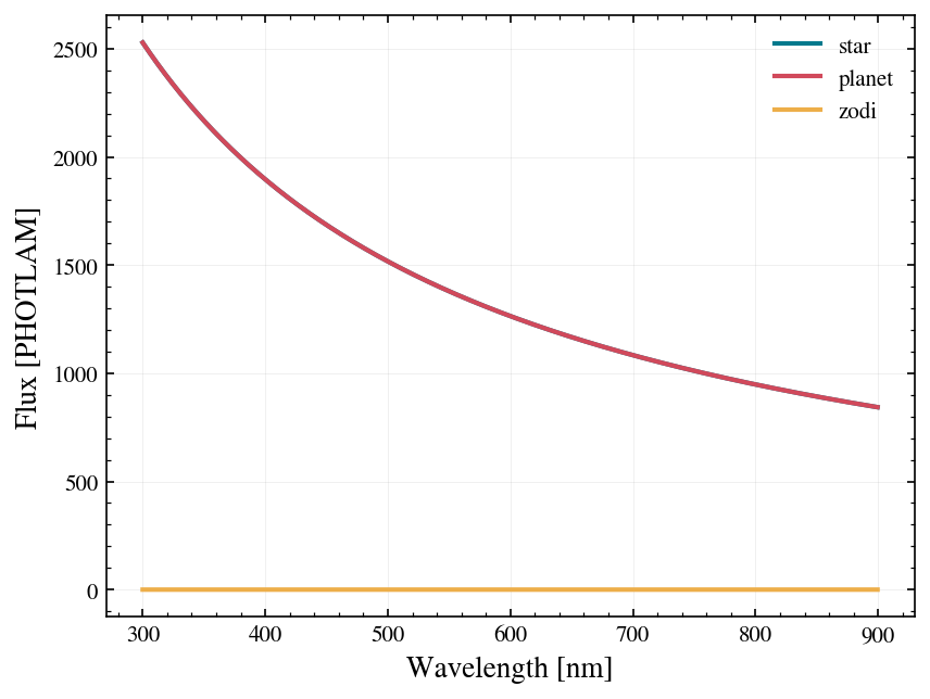
get_scene builds the star, planet, zodi and exozodi elements. The star and planet magnitudes are Vega magnitudes in the ESC band by default; hoststar_band= and mag_system= change that. The coronagraph carries the raw dark-hole contrast, the post-processing gain and the planet separation.

scene = get_scene(t, hoststarmag=-0.353, planetdeltamag=20, bg_flux=22.5, exobg_flux=21)
c = Coronagraph.from_default(t, raw_dh_contrast=1e-8, ppgain=10, separation=0.2)
print('star mag    :', scene.star.mag, scene.star.mag_system)
print('planet dmag :', scene.planet.deltamag)
print('contrast    :', c.raw_dh_contrast, '| ppgain', c.ppgain, '| separation', c.separation, 'arcsec')

fig, ax = scene.plot_spectra()

star mag    : -0.353 vega
planet dmag : 20
contrast    : 1e-08 | ppgain 10 | separation 0.2 arcsec

5. Assemble by hand

from_components gives the same object from_default would have built.

sim = Simulation.from_components(t, s, scene, c)
base = sim.get_snr(3600, 100)['snr']
print('SNR:', round(base, 3))
assert abs(base - Simulation.from_default().get_snr(3600, 100)['snr']) < 1e-9

SNR: 9.747

6. Change parameters

update() changes a parameter in place and the next calculation sees it. From the simulation, nested parameters are addressed with double underscores, so sim.update(coronagraph__ppgain=100) is the same as sim.coronagraph.update(ppgain=100). An invalid value is refused and leaves the object unchanged. sim.reset() puts every component back to its initial state.

Two changes below, one at a time. A fainter host means a fainter planet, because the planet is defined relative to the host, so the SNR drops and the curve is no longer near its plateau. Raising ppgain then lifts the plateau from 10 to 100 and the SNR climbs back most of the way, but not above the default scene’s: the fainter planet is photon-limited rather than speckle-limited, so a higher plateau helps less than it would for the bright host.

sim.update(scene__star__mag=2.0)
faint = sim.get_snr(3600, 100)['snr']
print('host 2.35 mag fainter        :', round(faint, 3))
sim.update(coronagraph__ppgain=100)
faint_pp = sim.get_snr(3600, 100)['snr']
print('... and post-processing gain 100:', round(faint_pp, 3))
assert faint < faint_pp < base

try:
    sim.update(sensor__encircled_energy=1.7)
except ValueError as err:
    print('refused:', err)

sim.reset()
print('after reset:', round(sim.get_snr(3600, 100)['snr'], 3))
assert abs(sim.get_snr(3600, 100)['snr'] - base) < 1e-9

host 2.35 mag fainter        : 6.731
... and post-processing gain 100: 9.064
refused: encircled_energy must be in (0, 1], got 1.7
after reset: 9.747

Notebook 03 looks at what the three coronagraph parameters do to the SNR curve.