Note

This page is generated from the Jupyter notebook notebooks/01_getting_started.ipynb in the repository. You can download it and run it interactively.

Getting started with the WCC ETC

The Wide-field Context Camera (WCC) exposure time calculator estimates the signal-to-noise ratio (SNR) a source reaches in a given exposure. Every calculation has the same three steps:

1. Build a scene: the astrophysical source plus its background.

2. Build a simulation: the scene paired with a sensor, a filter, and the telescope.

3. Ask the simulation for an SNR, an exposure time, a peak-pixel value, or an image.

This notebook walks through those steps once. The other tutorials go deeper on saturation, PSFs, exposure-time inversion, source spectra, and host galaxies.

import matplotlib.pyplot as plt
import numpy as np

import wcc_etc

wcc_etc.set_wcc_style()

1. Build a scene

get_scene returns what you want to observe together with its background. Here it is a Sun-like G5V star at r = 20 on the zodiacal background. The name can be a Pickles spectral type ('G5V', 'K3IV', …), a parametric spectrum ('blackbody', 'flat', 'powerlaw', 'emission'), or a bundled template such as the 'hsiao07' SN Ia. bandpass sets the filter the magnitude refers to.

scene = wcc_etc.get_scene(
    name="G5V",
    mag=20,
    background="zodi",
    bandpass="johnson_r",
    background_prop={"bandpass": "johnson_r", "mag": 22.5},
)
scene

<wcc_etc.scene.Scene at 0x73d5afea5910>

2. Build a simulation for a sensor and filter

Simulation.from_sensor_and_scene pairs the scene with a detector and filter given as a kind:band label ('sony:r', 'sony:bb', 'qcmos:r'). Pixel size, gain, read noise, dark current and filter throughput all come from the bundled configuration files; the Lazuli telescope is attached automatically.

sim = wcc_etc.Simulation.from_sensor_and_scene("sony:r", scene)

print("pixel size :", sim.sensor.pixel_size)
print("bit depth  :", sim.sensor.bit_depth, "bit")
print("read noise :", sim.sensor.read_noise)

pixel size : 3.76 um / pix
bit depth  : 16 bit
read noise : 3.0442890448219115 electron / pix

3. Compute the SNR

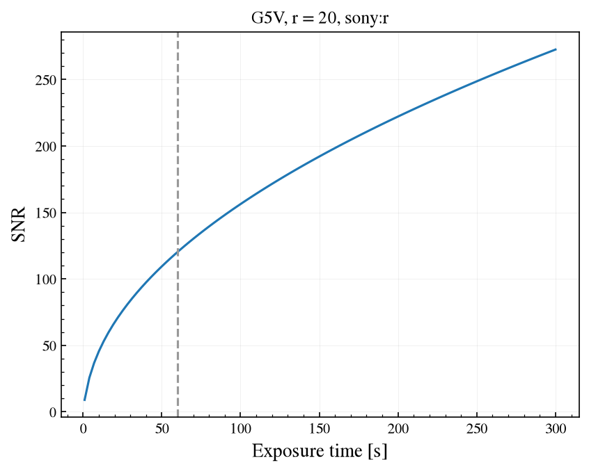
get_snr(time) renders the source through the PSF, does aperture photometry on the result, and returns a dict whose ["snr"] entry is the signal-to-noise ratio. The time can be a scalar or an array, so one call gives a whole SNR-vs-time curve.

sim.plot_snr(times) draws that curve. Like every plot method in the package it accepts an ax= to draw on and returns (fig, ax), so you can keep styling the axis afterwards.

times = np.linspace(1, 300, 100)
print(f"SNR at 60 s: {sim.get_snr(60)['snr']:.1f}")

fig, ax = sim.plot_snr(times)
ax.axvline(60, ls="--", color="0.6")
ax.set_title("G5V, r = 20, sony:r")
plt.show()

[wcc_etc] note: even n_pixels is rounded up by 1 to center the PSF peak (shown once).

SNR at 60 s: 120.2

4. Inspect and change parameters

sim.mutable_parameters lists every tunable parameter and sim.meta holds the current values. sim.update(**kwargs) changes them in place. A double underscore reaches into a nested field, so source__mag is the source magnitude inside the scene. A partial key works when it is unambiguous: jitter_sigma= resolves to telescope__jitter_sigma because nothing else ends that way. An ambiguous key such as mag= raises KeyError, since both the source and the background have one.

Two magnitudes of extra brightness is a factor of 6.3 in flux. The SNR rises by a factor of about 2.5 (here from 120 to 307), the square root of that, which is what you expect when the source’s own photon noise dominates the error budget.

Jitter is a second example. Switching the telescope’s 10 mas pointing jitter off sharpens the PSF, which raises the peak-pixel fraction by about 30 percent, yet the SNR barely moves: jitter shuffles light around inside the aperture rather than out of it.

print("mutable parameters:", sim.mutable_parameters[:8], "...")

before = float(sim.get_snr(60)["snr"])
sim.update(source__mag=18)  # brighter source
after = float(sim.get_snr(60)["snr"])

print(f"SNR @ 60 s, r = 20 : {before:.1f}")
print(f"SNR @ 60 s, r = 18 : {after:.1f}")

# The telescope carries 10 mas of pointing jitter by default.
sim.update(telescope__jitter_sigma=0)
print(f"SNR @ 60 s, r = 18, jitter off : {float(sim.get_snr(60)['snr']):.1f}")
print(f"peak-pixel fraction, jitter off : {sim.peak_pixel_fraction():.4f}")
sim.update(telescope__jitter_sigma=10)
print(f"peak-pixel fraction, 10 mas     : {sim.peak_pixel_fraction():.4f}")

mutable parameters: ['time', 'r_aper_mas', 'n_reads', 'telescope__f_num', 'telescope__diameter_primary', 'telescope__jitter_sigma', 'sensor__bandpass', 'sensor__bandpass_name'] ...
SNR @ 60 s, r = 20 : 120.2
SNR @ 60 s, r = 18 : 306.7
SNR @ 60 s, r = 18, jitter off : 307.3
peak-pixel fraction, jitter off : 0.1228
peak-pixel fraction, 10 mas     : 0.0956

5. Check what you actually set up

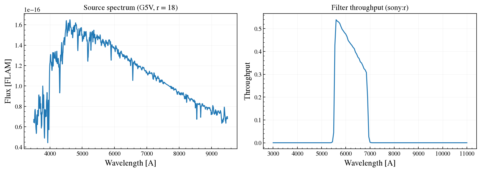
The scene source and the sensor both draw themselves. This is the quickest check that you built the source and filter you intended. plot and show are the same method on these objects.

fig, (ax_src, ax_filt) = plt.subplots(1, 2, figsize=(11, 4))

sim.scene.source.plot(ax=ax_src, wave=np.arange(3500, 9500, 5.0), flux_unit="flam")
ax_src.set_title("Source spectrum (G5V, r = 18)")

sim.sensor.plot(ax=ax_filt)
ax_filt.set_title("Filter throughput (sony:r)")

fig.tight_layout()
plt.show()

Summary

• get_scene(name, mag, background, bandpass) builds the scene; Simulation.from_sensor_and_scene("kind:band", scene) attaches the detector, filter and telescope.

• sim.get_snr(time)["snr"] is the SNR; time broadcasts, and sim.plot_snr(times) draws the curve.

• sim.update(source__mag=...) changes any mutable parameter in place; ambiguous keys raise KeyError.

• sim.scene.source.plot() and sim.sensor.plot() show the spectrum and the filter you set up.

Where to go next

Notebook	What it adds
02_saturation_flag.ipynb	Peak-pixel values and the saturation ceiling.
03_from_sensorfilter.ipynb	Canonical kind:band labels with the PSF picked from the filter’s focus level.
04_psf_and_image_snr.ipynb	PSF models, simulated images, and the PSF-aware SNR with aperture optimization.
05_n_reads_exptime.ipynb	Exposure time for a target SNR, and what multiple reads cost.
06_source_spectra.ipynb	Parametric source spectra and the normalization bandpass.
07_sersic_host.ipynb	A transient on a Sersic-profile host galaxy.