Note

This page is generated from the Jupyter notebook notebooks/05_n_reads_exptime.ipynb in the repository. You can download it and run it interactively.

n_reads and the exposure-time inverses

Two related Simulation capabilities:

• The exposure-time inverse. get_image_exptime_for_snr(snr) answers how long to integrate to reach a target SNR, inverting get_image_snr. The older analytic get_exptime_for_snr is deprecated and kept for cross-checks.

• Multiple reads. n_reads splits one exposure into frames. Read noise is paid once per frame, and saturation is judged on a single frame.

import matplotlib.pyplot as plt
import numpy as np

import wcc_etc


def make_sim(mag, sensor="sony:r"):
    """A G5V source of the given magnitude on the standard zodi background."""
    scene = wcc_etc.get_scene(
        name="G5V",
        mag=mag,
        background="zodi",
        bandpass="johnson_r",
        background_prop={"bandpass": "johnson_r", "mag": 22.5},
    )
    return wcc_etc.Simulation.from_sensor_and_scene(sensor, scene)


wcc_etc.set_wcc_style()
sim = make_sim(20)

1. How long to reach a target SNR

get_image_exptime_for_snr returns a dict whose 'time_s' is the answer, alongside the aperture it solved for. plot_exptime_for_snr draws it for a grid of targets. The required time grows as SNR squared, and each magnitude of extra faintness costs another factor of 2.5 in time at these magnitudes, where the source’s own photon noise dominates. In the background-limited regime, further down, the factor per magnitude becomes 6.3.

targets = np.linspace(10, 200, 25)

fig, ax = plt.subplots(figsize=(7, 4.2))
for mag in (19, 20, 21):
    make_sim(mag).plot_exptime_for_snr(targets, ax=ax, label=f"r = {mag}")
ax.set_title("Time to reach a target SNR (G5V, sony:r)")
plt.show()

res = sim.get_image_exptime_for_snr(100.0)
print(f"r = 20, SNR = 100 needs {res['time_s']:.1f} s")
print(f"  aperture radius   : {res['r_aper_mas']:.1f} mas")
print(f"  enclosed fraction : {res['enclosed_fraction']:.3f}")
print(f"  noise pixels      : {res['n_pix']}")

[wcc_etc] note: even n_pixels is rounded up by 1 to center the PSF peak (shown once).

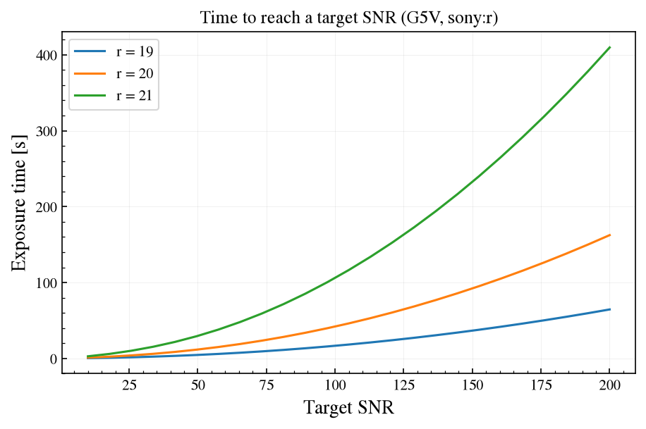
r = 20, SNR = 100 needs 42.1 s
  aperture radius   : 69.6 mas
  enclosed fraction : 0.882
  noise pixels      : 57

2. The cost of more reads

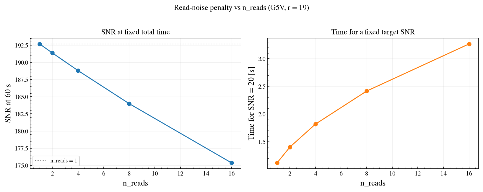
At a fixed total time the read noise is incurred once per frame, so the SNR falls with n_reads, and the time needed for a fixed target SNR grows. The effect is largest for a faint source where read noise matters, so this uses r = 19, where going from 1 to 16 reads costs about 9 percent of the SNR at 60 s.

plot_sweep evaluates the SNR for each value of any update() key and restores the original value afterwards. The time-for-SNR panel loops by hand.

faint = make_sim(19)
reads = [1, 2, 4, 8, 16]
fixed_t, snr_goal = 60.0, 20.0

snr_one_read = float(faint.get_snr(fixed_t)["snr"])

fig, (ax_snr, ax_t) = plt.subplots(1, 2, figsize=(11, 4.2))
faint.plot_sweep("n_reads", reads, time=fixed_t, ax=ax_snr, marker="o")
ax_snr.axhline(snr_one_read, color="grey", ls=":", lw=1, label="n_reads = 1")
ax_snr.set_ylabel(f"SNR at {fixed_t:.0f} s")
ax_snr.set_title("SNR at fixed total time")
ax_snr.legend(fontsize=9)

t_vs_reads = []
for n in reads:
    faint.update(n_reads=n)
    t_vs_reads.append(faint.get_image_exptime_for_snr(snr_goal)["time_s"])
faint.update(n_reads=1)

faint.update(n_reads=reads[-1])
snr_many = float(faint.get_snr(fixed_t)["snr"])
faint.update(n_reads=1)
print(
    f"SNR at {fixed_t:.0f} s: {snr_one_read:.1f} with 1 read, "
    f"{snr_many:.1f} with {reads[-1]} reads "
    f"({100 * (1 - snr_many / snr_one_read):.0f}% lower)"
)

ax_t.plot(reads, t_vs_reads, "o-", color="C1")
ax_t.set_xlabel("n_reads")
ax_t.set_ylabel(f"Time for SNR = {snr_goal:.0f} [s]")
ax_t.set_title("Time for a fixed target SNR")

fig.suptitle("Read-noise penalty vs n_reads (G5V, r = 19)", y=1.02)
fig.tight_layout()
plt.show()

SNR at 60 s: 192.7 with 1 read, 175.4 with 16 reads (9% lower)

3. Reads as a saturation escape hatch

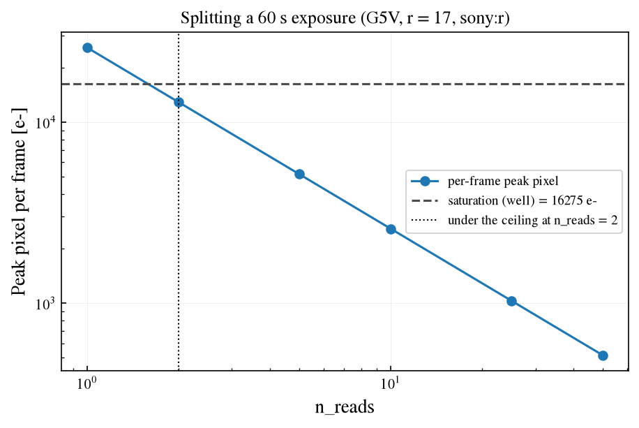
Saturation is evaluated on a single t / n_reads frame, so the per-frame peak falls as 1 / n_reads. A bright star that clips in one long frame can be brought back under the ceiling by splitting the same total time across more reads. The ceiling here is sensor.saturation_e, the full well on the Sony.

bright = make_sim(17)
total_t = 60.0
sat_reads = np.array([1, 2, 5, 10, 25, 50])

peaks = []
for n in sat_reads:
    bright.update(n_reads=int(n))
    peaks.append(bright.get_peak_pixel(total_t, units="e-").value)
bright.update(n_reads=1)
peaks = np.array(peaks)

ceiling = bright.sensor.saturation_e.value
below = sat_reads[peaks < ceiling]

fig, ax = plt.subplots(figsize=(7, 4.2))
ax.loglog(sat_reads, peaks, "o-", label="per-frame peak pixel")
limit = bright.sensor.saturation_limit
ax.axhline(
    ceiling, color="0.3", ls="--", label=f"saturation ({limit}) = {ceiling:.0f} e-"
)
if below.size:
    ax.axvline(
        below[0],
        color="k",
        ls=":",
        lw=1,
        label=f"under the ceiling at n_reads = {below[0]}",
    )
ax.set_xlabel("n_reads")
ax.set_ylabel("Peak pixel per frame [e-]")
ax.set_title(f"Splitting a {total_t:.0f} s exposure (G5V, r = 17, sony:r)")
ax.legend(fontsize=9)
plt.show()

Summary

• get_image_exptime_for_snr inverts the PSF-aware SNR and reports the aperture it solved for; plot_exptime_for_snr draws it for a grid of targets. The analytic get_exptime_for_snr is deprecated but still available as a cross-check.

• n_reads splits the total exposure into frames and pays the read noise once per frame: at fixed time the SNR drops, and the time for a target SNR grows. plot_sweep("n_reads", ...) shows the first of those in one call.

• Saturation is judged per frame, so more reads lower the per-frame peak and can bring a clipping star back under sensor.saturation_e.