PSFs and image simulation

wcc-etc can render a detector image of the scene with the point-spread function, telescope jitter, sky background, Poisson and read noise, and per-pixel saturation.

PSF models

All PSF models subclass PSFSource and implement render(ctx) and cache_key():

Class	Description
`AiryPSF`	Diffraction-limited Airy disk computed for the simulation’s source-weighted effective wavelength, plate scale and aperture. The default when no PSF is given.
`PolychromaticPSF`	A photon-weighted coadd of a base PSF rendered at several wavelengths across the band. Build one with `polychromatic_psf()`.
`DefocusPSF`	A resampled Zemax Huygens PSF loaded from disk. Two defocus products ship with the package (see below).
`CustomPSF`	An arbitrary PSF from a NumPy array or a file, with a given source pixel scale (`src_um_per_pix`).

The wavelength the PSF is rendered at

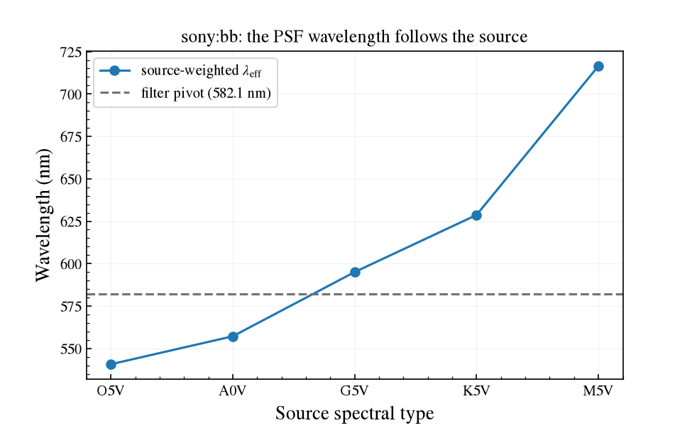
The diffraction scale is linear in wavelength, so which wavelength stands in for a broad band matters. wcc-etc renders the PSF at the source-weighted effective wavelength

\[\lambda_\mathrm{eff} = \frac{\int \lambda\, S(\lambda)\, T(\lambda)\, d\lambda} {\int S(\lambda)\, T(\lambda)\, d\lambda},\]

with \(S\) the source photon flux density and \(T\) the total throughput. It is available as effective_wavelength and as the standalone wcc_etc.effective_wavelength():

from wcc_etc import effective_wavelength

sim.effective_wavelength                                    # <Quantity 716.5 nm>
effective_wavelength(sim.sensor.bandpass, spectrum)         # the same, standalone

This is deliberately different from sensor.wavelength, the filter pivot wavelength. The pivot is computed from the throughput curve alone, so it is the same for every source: the WCC broad band has a pivot of 582.1 nm whether the star is an O5V or an M5V. Weighting by the SED as well moves it by more than 150 nm across the main sequence, and with it the modelled central-pixel fraction (sony:bb, 10 mas jitter):

Source	Filter pivot	\(\lambda_\mathrm{eff}\)	Central-pixel fraction	Error at pivot
O5V	582.1 nm	540.7 nm	0.1140	−9.4 %
A0V	582.1 nm	557.1 nm	0.1096	−5.7 %
G5V	582.1 nm	595.0 nm	0.1002	+3.1 %
K5V	582.1 nm	628.7 nm	0.0926	+11.5 %
M5V	582.1 nm	716.5 nm	0.0762	+35.6 %

The last column is the error of a render at the pivot, which predicts 0.1033 for every one of these sources. For an M5V that overpredicts the brightest pixel by 36 % and so predicts saturation well before it happens, and it underpredicts for blue sources. WCC’s purpose is broadband context imaging, so the broad bands are the common case.

import matplotlib.pyplot as plt
import wcc_etc
from wcc_etc import (
    get_scene, Simulation, ImageSimulator, AiryPSF, DefocusPSF,
    DEFOCUS_1WAVE_PATH, DEFOCUS_2WAVE_PATH, plot_image_mpl, plot_radial_mpl,
)

wcc_etc.set_wcc_style()

TYPES = ["O5V", "A0V", "G5V", "K5V", "M5V"]
lam_eff = []
for spectral_type in TYPES:
    scene_st = get_scene(
        spectral_type, mag=12, background="zodi", bandpass="johnson_r"
    )
    sim_st = Simulation.from_sensor_and_scene("sony:bb", scene_st)
    lam_eff.append(sim_st.effective_wavelength.to_value("nm"))

pivot = sim_st.sensor.wavelength.to_value("nm")

fig, ax = plt.subplots(figsize=(6.5, 4.0))
ax.plot(TYPES, lam_eff, "o-", label=r"source-weighted $\lambda_\mathrm{eff}$")
ax.axhline(
    pivot, ls="--", color="0.45", label=f"filter pivot ({pivot:.1f} nm)"
)
ax.set_xlabel("Source spectral type")
ax.set_ylabel("Wavelength (nm)")
ax.set_title("sony:bb: the PSF wavelength follows the source")
ax.legend()

Polychromatic PSFs

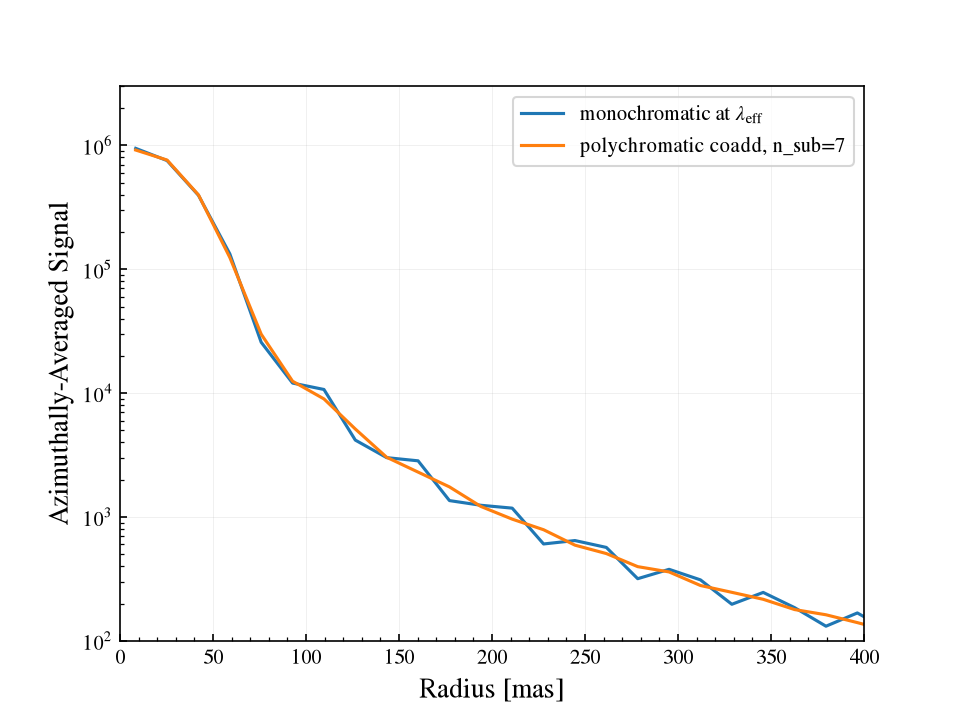
Rendering at \(\lambda_\mathrm{eff}\) fixes the PSF width, but the result is still a single monochromatic PSF with diffraction rings at full contrast. For the real broadband shape, coadd renders across the band with polychromatic_psf():

psf = sim.polychromatic_psf(n_sub=7)     # 7 equal-photon-weight sub-bands
sim.get_image_snr(time=30, psf=psf)
sim.get_peak_pixel(30, psf=psf)

The sub-band edges sit at equal quantiles of the cumulative photon weight (wcc_etc.photon_weighted_subbands()), so the samples cluster where the source delivers light and no render is spent on a negligible sub-band. n_sub=1 reduces exactly to the monochromatic \(\lambda_\mathrm{eff}\) case. Five to nine sub-bands is plenty for a broad optical band, and the cost is linear in n_sub. The effect on the central-pixel fraction is a few percent, since a coadd of narrower and wider PSFs peaks slightly above the PSF at the mean wavelength, so this is a refinement on top of the \(\lambda_\mathrm{eff}\) choice and not a second large correction.

On an M5V source the coadd fills in the monochromatic diffraction minima and takes the tops off the maxima, while leaving the overall width alone. The comparison below switches jitter off (jitter_sigma_mas=0) and zooms into the core. At the telescope’s real jitter the ring structure is smeared out and the two profiles lie on top of each other:

scene_m5 = get_scene("M5V", mag=12, background="zodi", bandpass="johnson_r")
sim_m5 = Simulation.from_sensor_and_scene("sony:bb", scene_m5)
imsim_m5 = ImageSimulator.from_sensor_and_scene("sony:bb", scene_m5, npix=200)

mono = imsim_m5.simulate(
    time=30, psf=AiryPSF(), add_noise=False, jitter_sigma_mas=0.0
)
poly = imsim_m5.simulate(
    time=30, psf=sim_m5.polychromatic_psf(n_sub=7),
    add_noise=False, jitter_sigma_mas=0.0,
)

fig, ax = plt.subplots()
plot_radial_mpl(mono, units="mas", ax=ax, show_hwhm=False)
plot_radial_mpl(poly, units="mas", ax=ax, show_hwhm=False)
ax.lines[0].set_label(r"monochromatic at $\lambda_\mathrm{eff}$")
ax.lines[1].set_label("polychromatic coadd, n_sub=7")
ax.set_yscale("log")
ax.set_xlim(0, 400)
ax.set_ylim(1e2, 3e6)
ax.legend()

Bundled defocus PSFs

Two Zemax Huygens PSFs (1 and 2 waves of defocus, computed at 500 nm and f/15 with 4 µm data spacing) ship with the package as FITS products and are exposed as path constants:

from wcc_etc import DefocusPSF, DEFOCUS_1WAVE_PATH, DEFOCUS_2WAVE_PATH

psf1 = DefocusPSF(DEFOCUS_1WAVE_PATH)   # 1-wave defocus
psf2 = DefocusPSF(DEFOCUS_2WAVE_PATH)   # 2-wave defocus

The FITS headers carry PIXSCALE (µm/sample), WAVELEN (the reference wavelength, nm), FNUM (the reference f-number) and DEFOCUSW (the defocus in waves), so DefocusPSF needs no hand-passed sampling and can map the array onto the optics it is asked about. A new Huygens .txt export is turned into such a product with wcc_etc.psfsim.huygens_txt_to_fits().

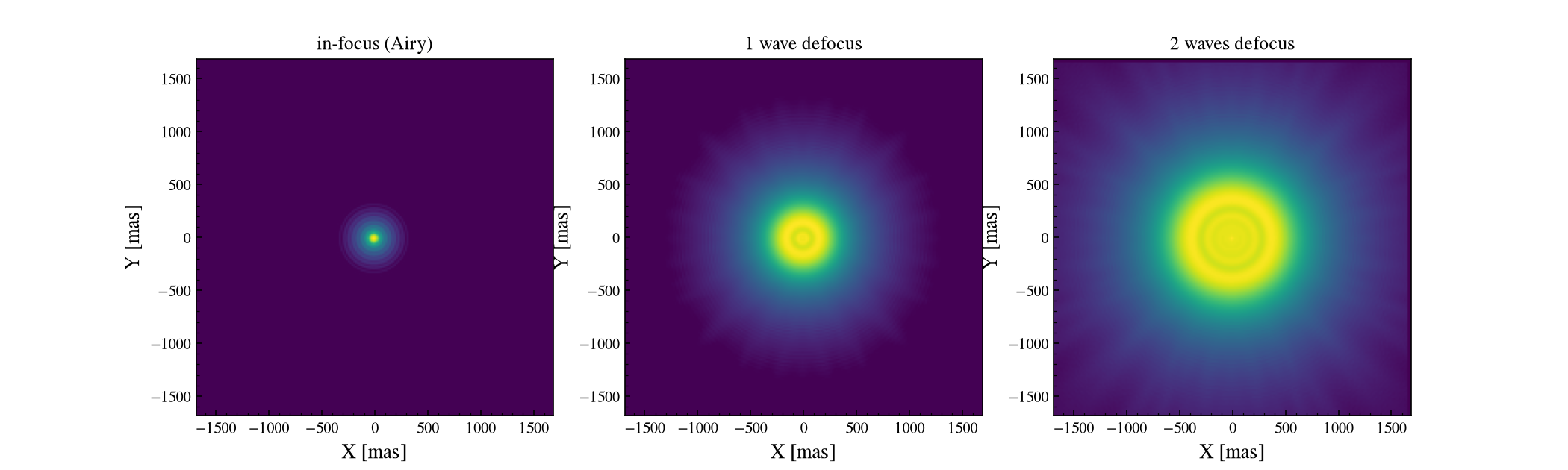
This is what the two products look like on the detector, against an in-focus Airy PSF for scale (noiseless, same source and exposure in each panel):

scene_g5 = get_scene("G5V", mag=12, background="zodi", bandpass="johnson_r")
imsim_g5 = ImageSimulator.from_sensor_and_scene("sony:r", scene_g5, npix=200)

panels = [
    ("in-focus (Airy)", AiryPSF()),
    ("1 wave defocus", DefocusPSF(DEFOCUS_1WAVE_PATH)),
    ("2 waves defocus", DefocusPSF(DEFOCUS_2WAVE_PATH)),
]

fig, axes = plt.subplots(1, 3, figsize=(14, 4.2))
for ax, (label, psf) in zip(axes, panels):
    image = imsim_g5.simulate(time=30, psf=psf, add_noise=False)
    plot_image_mpl(image, ax=ax, units="mas", colorbar=False, title=label)

How a resampled PSF is scaled

A sampled PSF array was computed for one wavelength and one f-number, so rendering it onto a detector means deciding how its spatial scale maps onto the optics in hand. DefocusPSF and CustomPSF take a wavelength_scaling argument for that. A defocus blur diameter is \(\Delta z / F\#\), with \(\Delta z\) the longitudinal focus error:

Mode	Meaning
`"despace"`	The default. A fixed longitudinal focus error, such as a mechanical despace or a filter substrate of a given thickness in the converging beam. \(\Delta z\) is then a fixed distance, so the blur diameter \(\Delta z / F\#\) has no wavelength dependence, and source colour only alters the fine diffraction structure inside the blur (a second-order effect at these Strehl ratios: 0.011 for the 1-wave product). Scale factor \(F\#_\mathrm{ref} / F\#\).
`"waves"`	A defocus held at a constant number of waves of wavefront error at every wavelength: \(\Delta z = 8 W \lambda F\#^2\), so the blur diameter is \(8 W \lambda F\#\). Scale factor \((\lambda / \lambda_\mathrm{ref})(F\# / F\#_\mathrm{ref})\). Use this if your product’s defocus is specified as a wavefront error rather than as a distance.
`"none"`	Render at the array’s native sampling, ignoring `ctx.wavelength_m` and `ctx.fnum`. Must be requested explicitly.

Both metadata-driven modes agree at the wavelength and f-number the product was computed at. A PSF that carries no reference metadata raises instead of silently ignoring the optics it was handed:

CustomPSF(array, src_um_per_pix=4.0).render(ctx)
# ValueError: ... cannot apply wavelength_scaling='despace' without
# ref_wavelength_m and ref_fnum ...

Custom PSFs

Declare the optics the array was computed for, or opt out of scaling explicitly:

import numpy as np
from wcc_etc import CustomPSF

array = np.load("my_psf.npy")

# tracks the optics it is rendered onto
psf = CustomPSF(array, src_um_per_pix=4.0, ref_wavelength_m=500e-9, ref_fnum=15.0)

# or: render at native sampling, whatever the optics
psf = CustomPSF(array, src_um_per_pix=4.0, wavelength_scaling="none")

Automatic PSF selection by focus level

When you build a simulation with from_sensorfilter(), the default PSF for that sensor and filter, in focus or defocused, is used whenever you omit psf= in simulate, render_psf, get_image_snr and get_image_exptime_for_snr. Read it back with default_psf, which falls back to a diffraction-limited AiryPSF for simulations built any other way:

sim = Simulation.from_sensorfilter("zwo:bb2", scene)
type(sim.default_psf).__name__        # 'DefocusPSF'

Rendering a PSF on its own

render_psf() returns the bare PSF on the detector grid, normalized to unit sum, with no source flux, background or noise. It is the right tool for comparing PSF shapes, peak-pixel fractions, radial profiles and encircled energy across focus levels or jitter values. Because it builds its render context the same way simulate does, it honours the source-weighted \(\lambda_\mathrm{eff}\) described above. plot_psf() draws that render as an image with a log stretch.

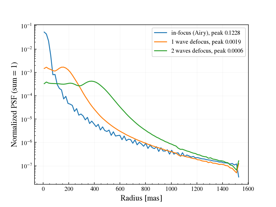
Pair render_psf with plate_scale_mas to feed the plotting helpers in milliarcseconds. The peak of the normalized PSF is the central-pixel fraction that sets when the detector saturates. Here it falls by a factor of about 200 from in-focus to two waves of defocus:

imsim_r = ImageSimulator.from_sensor_and_scene("sony:r", scene_g5, npix=200)

fig, ax = plt.subplots()
for label, psf in panels:
    psf_img = imsim_r.render_psf(psf, jitter_sigma_mas=0.0, npix=128)
    plot_radial_mpl(
        image_clean=psf_img,
        pixel_scale_mas=imsim_r.plate_scale_mas,
        units="mas",
        ax=ax,
        show_hwhm=False,
        label=f"{label}, peak {psf_img.max():.4f}",
    )
ax.set_yscale("log")
ax.set_xlabel("Radius [mas]")
ax.set_ylabel("Normalized PSF (sum = 1)")
ax.legend()

Simulating an image

Use ImageSimulator:

from wcc_etc import ImageSimulator, AiryPSF

imsim = ImageSimulator.from_sensor_and_scene("sony:r", scene, npix=300)
img = imsim.simulate(
    time=30,
    psf=AiryPSF(),
    jitter_sigma_mas=None,    # None → use the telescope's jitter
    add_noise=True,
    seed=0,                   # reproducible noise
)

simulate returns a SimulatedImage with:

Attribute / method	Description
`image_e`	Noisy image in electrons.
`image_clean`	Noiseless image (mean electrons).
`saturation_mask`	Boolean mask of saturated pixels.
`to_adu()`	Image converted to ADU using the sensor gain and bit depth.
`to_fitsimg()`	A `FitsImg` for aperture photometry and plotting.
`plot_image()` (also `plot`), `plot_image_row()`, `plot_radial()`, `plot_encircled_energy()`	Plotting dispatchers (see Plotting).

Grid size and oversampling

npix sets the rendered grid and must be large enough to contain the PSF. oversample controls sub-pixel rendering before binning to detector pixels. The default npix inside the SNR path (128) contains the bundled defocus PSFs for the current sensors, but very small pixels or stronger defocus may need a larger value.

Telescope jitter

Pointing jitter is applied as a Gaussian blur with standard deviation jitter_sigma_mas. Passing None uses the telescope’s configured jitter_sigma (10 mas for Lazuli by default); pass a value to override it for a single call.