Note

This page is generated from the Jupyter notebook notebooks/02_saturation_flag.ipynb in the repository. You can download it and run it interactively.

Saturation flagging

A source saturates when its brightest pixel reaches the detector’s saturation ceiling, sensor.saturation_e. That ceiling is the smaller of two numbers: the full well of the pixel, and the charge at which the ADC clips, (adc_max - bias_level) * gain. sensor.saturation_limit reports which of the two binds ("well" or "adc"). The peak-pixel budget adds the source PSF peak, the per-pixel sky, the dark current, and the bias.

Key API: sensor.saturation_e, sensor.saturation_limit, sim.peak_pixel_fraction(), sim.get_peak_pixel(time), sim.is_saturated(time), and sim.plot_peak_pixel(time).

import matplotlib.pyplot as plt
import numpy as np

import wcc_etc

wcc_etc.set_wcc_style()

scene = wcc_etc.get_scene(
    name="G5V",
    mag=15,
    background="zodi",
    bandpass="johnson_r",
    background_prop={"bandpass": "johnson_r", "mag": 22.5},
)

sim = wcc_etc.Simulation.from_sensor_and_scene("sony:r", scene)

What the detector can hold

On the Sony IMX455 the 16-bit ADC reaches 65535 ADU, but the full well of about 16 ke- fills first, so the well is the ceiling. peak_pixel_fraction() is the fraction of the total source flux landing in the single brightest pixel. It depends on wavelength, f-number, pixel size and jitter, and it is what turns a magnitude into a peak-pixel value.

s = sim.sensor
print(f"bit depth           : {s.bit_depth}")
print(f"adc_max             : {s.adc_max}")
print(f"full well           : {s.saturation_e:.0f}  (limit = {s.saturation_limit!r})")
print(f"ADC clip in e-      : {((s.adc_max - s.bias_level) * s.gain):.0f}")
print(f"peak pixel fraction : {sim.peak_pixel_fraction():.4f}")

bit depth           : 16
adc_max             : 65535.0 ct
full well           : 16275 electron  (limit = 'well')
ADC clip in e-      : 17118 electron
peak pixel fraction : 0.0956

[wcc_etc] note: even n_pixels is rounded up by 1 to center the PSF peak (shown once).

What saturation looks like

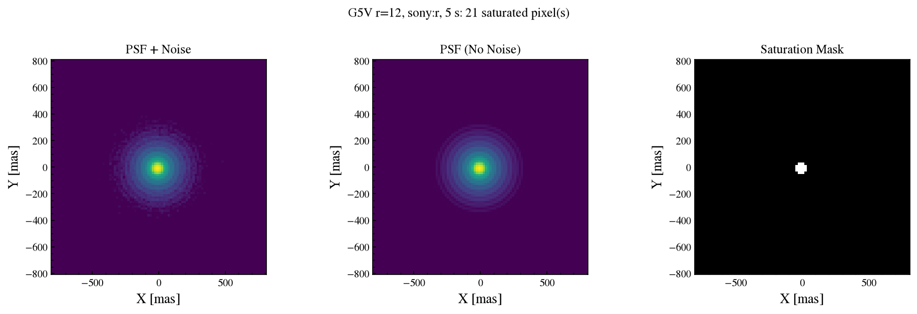
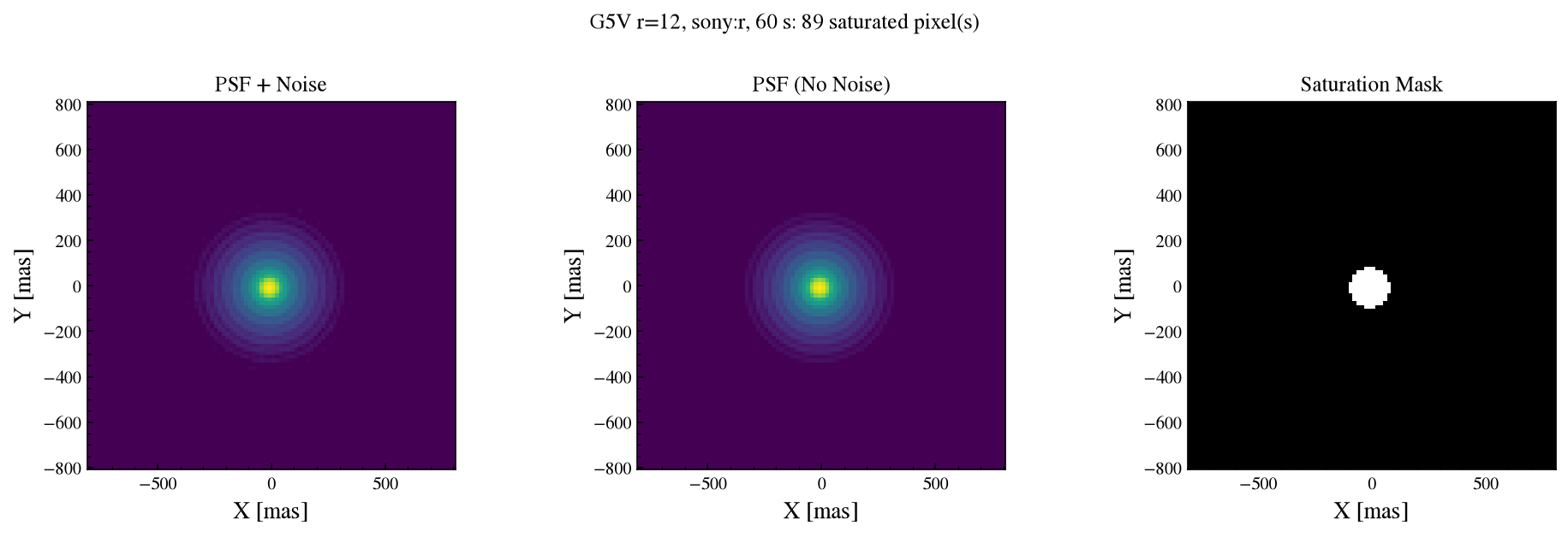
ImageSimulator.simulate returns a SimulatedImage carrying a saturation_mask, and plot_image_row shows the noisy image, the noiseless image, and that mask on a shared colour scale. At 5 s this r = 12 star is within range; at 60 s the core clips.

bright = wcc_etc.get_scene(
    name="G5V",
    mag=12,
    background="zodi",
    bandpass="johnson_r",
    background_prop={"bandpass": "johnson_r", "mag": 22.5},
)
imsim = wcc_etc.ImageSimulator.from_sensor_and_scene("sony:r", bright, npix=96)

for t in (5, 60):
    res = imsim.simulate(time=t, seed=0)
    fig, axes = res.plot_image_row(stretch="log", units="mas", figsize=(13, 4))
    fig.suptitle(
        f"G5V r=12, sony:r, {t} s: {res.saturation_mask.sum()} saturated pixel(s)",
        y=1.02,
    )
    fig.tight_layout()
    plt.show()

Onset vs exposure time

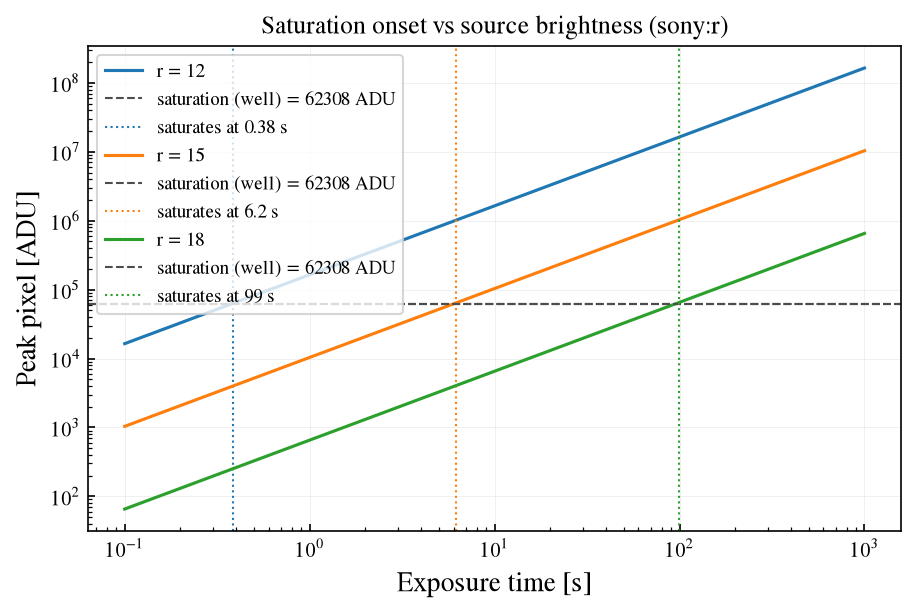
get_peak_pixel and is_saturated broadcast over an array of times, so the whole ramp up to the ceiling comes from one call each. plot_peak_pixel draws the ramp on log axes, dashes in the ceiling, and dots a vertical line at the first time is_saturated is true. Drawing three magnitudes on one axis is a loop over update; the legend names the onset time of each.

Each magnitude is a factor of 2.5 in flux, so the onset time moves by the same factor: three magnitudes fainter buys sixteen times longer before the core clips.

texp = np.logspace(-1, 3, 200)  # 0.1 s to 1000 s

fig, ax = plt.subplots(figsize=(7, 4.2))
for mag in (12, 15, 18):
    sim.update(source__mag=mag)
    sim.plot_peak_pixel(texp, ax=ax, label=f"r = {mag}")
    sat = sim.is_saturated(texp)
    onset = f"saturates after {texp[sat][0]:.2g} s" if sat.any() else "no saturation"
    print(f"r = {mag}: {onset}")
ax.set_title("Saturation onset vs source brightness (sony:r)")
ax.legend(fontsize=9)
plt.show()

sim.update(source__mag=15)

r = 12: saturates after 0.38 s
r = 15: saturates after 6.2 s
r = 18: saturates after 99 s

The ceiling depends on the sensor

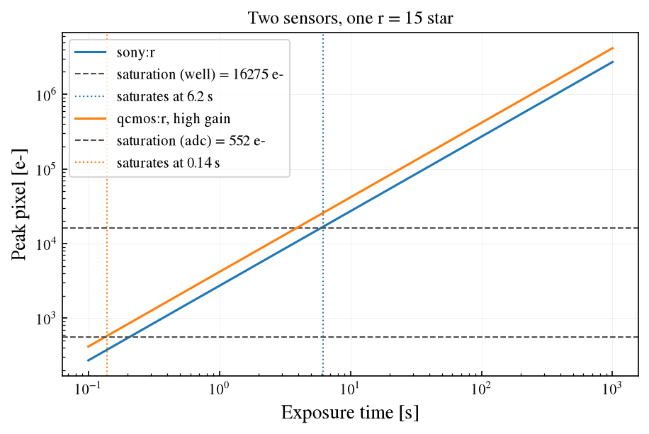
The qCMOS in its default high-gain mode has a 12-bit ADC (4095 ADU) and a gain of about 0.13 e-/ADU, so the ADC clips at only 552 e-, well below the full well. The same r = 15 star therefore saturates it far sooner than the Sony. Overlaying the two simulations shows both ceilings; each curve’s onset marker takes its own colour.

sim_q = wcc_etc.Simulation.from_sensor_and_scene("qcmos:r", scene)

fig, ax = plt.subplots(figsize=(7, 4.2))
for label, s in [("sony:r", sim), ("qcmos:r, high gain", sim_q)]:
    s.plot_peak_pixel(texp, ax=ax, units="e-", label=label)
    ceiling, limit = s.sensor.saturation_e, s.sensor.saturation_limit
    print(f"{label:<20} ceiling {ceiling:.0f} ({limit})")
ax.set_title("Two sensors, one r = 15 star")
plt.show()

sony:r               ceiling 16275 electron (well)
qcmos:r, high gain   ceiling 552 electron (adc)

Summary

• A source saturates when its peak pixel reaches sensor.saturation_e, the smaller of the full well and the ADC clip. sensor.saturation_limit says which one.

• sim.peak_pixel_fraction() converts a source magnitude into a peak-pixel value.

• sim.get_peak_pixel(time) and sim.is_saturated(time) broadcast over time; sim.plot_peak_pixel(time) draws the ramp with the ceiling and the onset.

• On the Sony the well binds; on the qCMOS in high gain the 12-bit ADC does.

• Saturation is judged on a single frame, so splitting an exposure into n_reads frames lowers the per-frame peak. Notebook 05 shows that.