Note

This page is generated from the Jupyter notebook notebooks/04_psf_and_image_snr.ipynb in the repository. You can download it and run it interactively.

PSF simulator and PSF-aware SNR

A tour of the detector-grid PSF simulator and the PSF-aware SNR:

• PSF sources: AiryPSF (diffraction limited), DefocusPSF (one or two waves, from Zemax Huygens data), and CustomPSF (any image).

• ImageSimulator: render_psf gives the bare normalized PSF, plot_psf draws it, and simulate builds a full detector image with sky, dark current, noise and a saturation mask.

• Simulation.get_image_snr: aperture photometry on the rendered PSF, with an optional search for the SNR-maximizing radius.

import matplotlib.pyplot as plt
import numpy as np

import wcc_etc

wcc_etc.set_wcc_style()

scene = wcc_etc.get_scene(
    name="G5V",
    mag=18,
    background="zodi",
    bandpass="johnson_r",
    background_prop={"bandpass": "johnson_r", "mag": 22.5},
)

sim = wcc_etc.Simulation.from_sensor_and_scene("sony:r", scene)
imsim = wcc_etc.ImageSimulator.from_sensor_and_scene("sony:r", scene, npix=300)

PSFS = {
    "Airy (diffraction limited)": wcc_etc.AiryPSF(),
    "+1 wave defocus": wcc_etc.DefocusPSF(wcc_etc.DEFOCUS_1WAVE_PATH),
    "+2 wave defocus": wcc_etc.DefocusPSF(wcc_etc.DEFOCUS_2WAVE_PATH),
}

print(f"plate scale : {imsim.plate_scale_mas:.1f} mas/pix")
print(f"aperture    : {sim.get_snr(60)['r_aper_mas']:.1f} mas (Airy default)")

plate scale : 16.9 mas/pix

[wcc_etc] note: even n_pixels is rounded up by 1 to center the PSF peak (shown once).

aperture    : 69.6 mas (Airy default)

1. PSF gallery

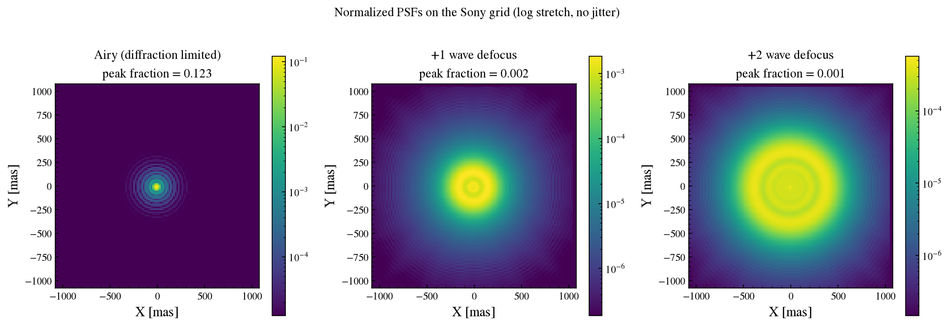
plot_psf renders a PSF onto the detector grid normalized to unit sum, with no source flux, background or noise, and draws it on a log stretch. Passing jitter_sigma_mas=0 switches off the pointing blur so the diffraction structure is visible. The peak of the normalized PSF is the peak-pixel fraction.

fig, axes = plt.subplots(1, 3, figsize=(13, 4.2))
for ax, (name, psf) in zip(axes, PSFS.items()):
    peak = sim.peak_pixel_fraction(psf=psf, jitter_sigma_mas=0.0)
    imsim.plot_psf(
        psf,
        ax=ax,
        jitter_sigma_mas=0.0,
        npix=128,
        title=f"{name}\npeak fraction = {peak:.3f}",
    )

fig.suptitle("Normalized PSFs on the Sony grid (log stretch, no jitter)", y=1.03)
fig.tight_layout()
plt.show()

2. A full detector image

simulate(time) distributes the source electrons over the PSF, adds the per-pixel sky and dark current, then Poisson and Gaussian read noise. The returned SimulatedImage carries image_clean, image_e, a saturation_mask, and the to_adu() and to_fitsimg() converters. plot_image_row shows all three arrays.

res = imsim.simulate(time=30, seed=0)

fig, axes = res.plot_image_row(stretch="log", units="mas")
fig.suptitle("G5V r=18, 30 s, sony:r, Airy PSF", y=1.02)
fig.tight_layout()
plt.show()

print(f"clean total electrons : {res.image_clean.sum():.3e}")
print(f"peak pixel (e-)       : {res.image_e.max():.1f}")
print(f"saturated pixels      : {res.saturation_mask.sum()}")

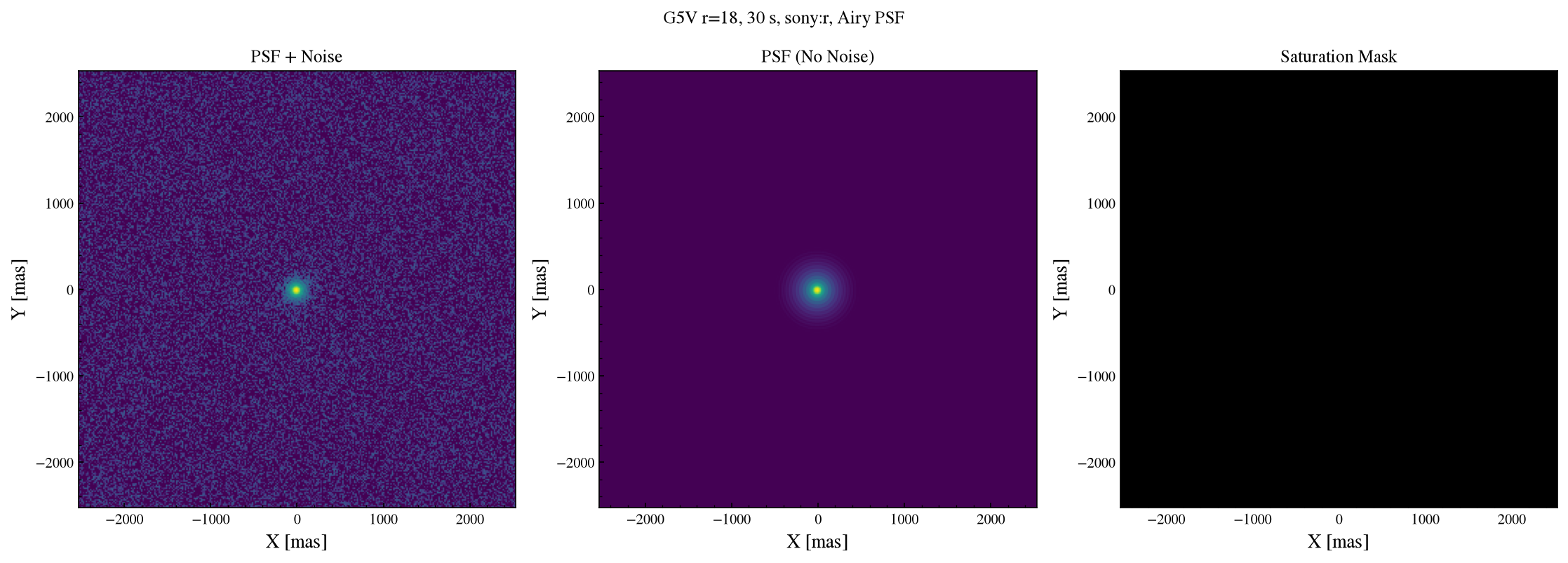
clean total electrons : 8.301e+04
peak pixel (e-)       : 5113.3
saturated pixels      : 0

Radial profile and encircled energy

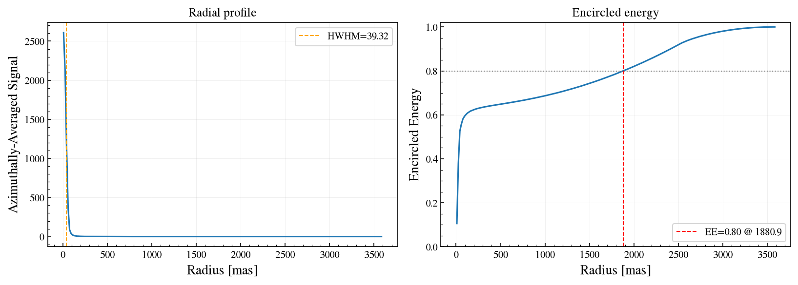
The same SimulatedImage plots its own azimuthally averaged radial profile and encircled-energy curve. plot_radial marks the half width at half maximum; plot_encircled_energy marks a target fraction.

fig, (ax_r, ax_ee) = plt.subplots(1, 2, figsize=(11, 4))
res.plot_radial(ax=ax_r, units="mas", title="Radial profile")
res.plot_encircled_energy(
    ax=ax_ee, units="mas", ee_target=0.8, title="Encircled energy"
)
fig.tight_layout()
plt.show()

Comparing focus levels

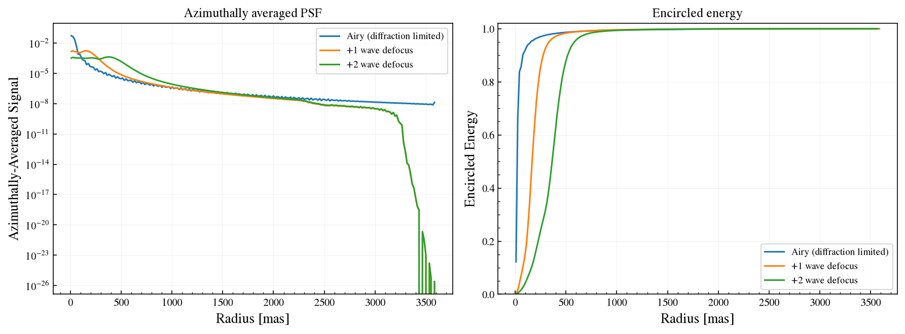
render_psf plus plate_scale_mas feed the same plotting helpers directly, so several normalized PSFs overlay on one axis. Defocus spreads the light into a broad doughnut: the radial peak drops by orders of magnitude and the encircled energy needs a much larger radius to reach the same fraction.

fig, (ax_r, ax_ee) = plt.subplots(1, 2, figsize=(12, 4.5))
for name, psf in PSFS.items():
    psf_img = imsim.render_psf(psf, jitter_sigma_mas=0.0)
    wcc_etc.plot_radial_mpl(
        image_clean=psf_img,
        pixel_scale_mas=imsim.plate_scale_mas,
        ax=ax_r,
        units="mas",
        show_hwhm=False,
        label=name,
    )
    wcc_etc.plot_encircled_energy_mpl(
        image_clean=psf_img,
        pixel_scale_mas=imsim.plate_scale_mas,
        ax=ax_ee,
        units="mas",
        ee_target=None,
        label=name,
    )

ax_r.set_yscale("log")
ax_r.set_title("Azimuthally averaged PSF")
ax_ee.set_title("Encircled energy")
ax_r.legend(fontsize=9)
ax_ee.legend(fontsize=9, loc="lower right")
fig.tight_layout()
plt.show()

3. Pointing jitter

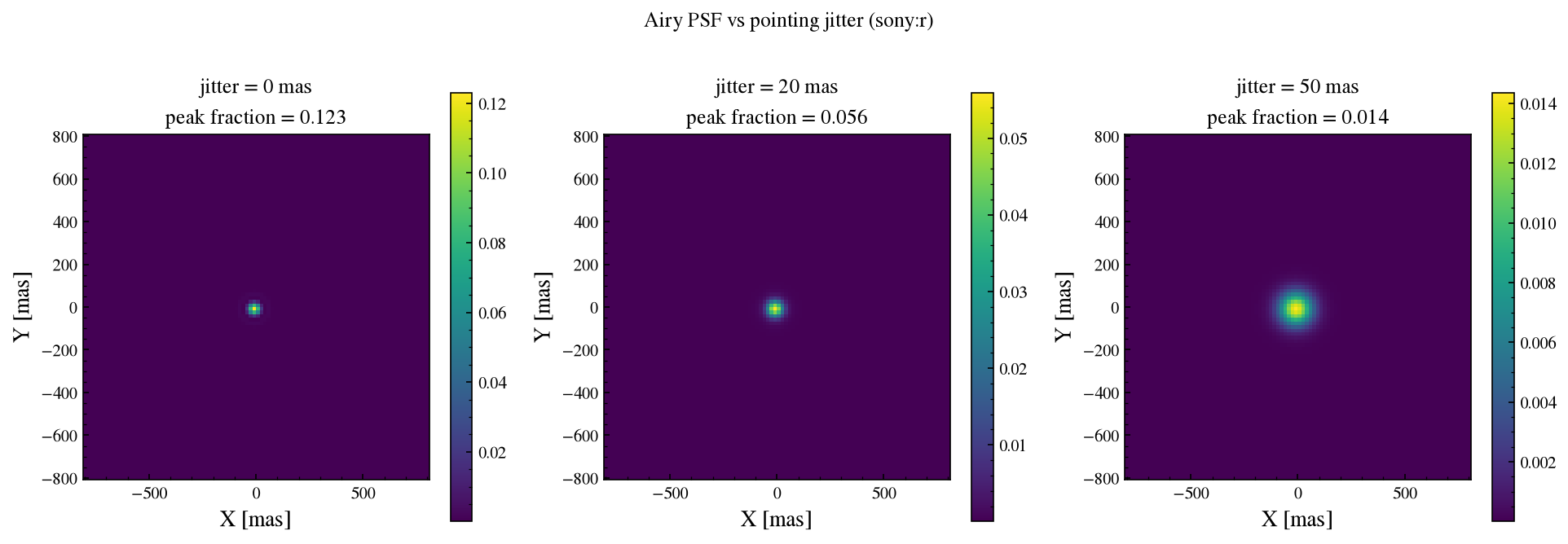
Jitter is a Gaussian blur of the PSF. More jitter means a broader core and a lower peak fraction, which is what drives the saturation budget in notebook 02. A linear stretch makes the change in the core easier to see.

fig, axes = plt.subplots(1, 3, figsize=(13, 4.2))
for ax, jitter in zip(axes, [0.0, 20.0, 50.0]):
    peak = sim.peak_pixel_fraction(jitter_sigma_mas=jitter)
    imsim.plot_psf(
        ax=ax,
        jitter_sigma_mas=jitter,
        npix=96,
        stretch="linear",
        title=f"jitter = {jitter:.0f} mas\npeak fraction = {peak:.3f}",
    )

fig.suptitle("Airy PSF vs pointing jitter (sony:r)", y=1.03)
fig.tight_layout()
plt.show()

4. Aperture size, defocus, and the optimum

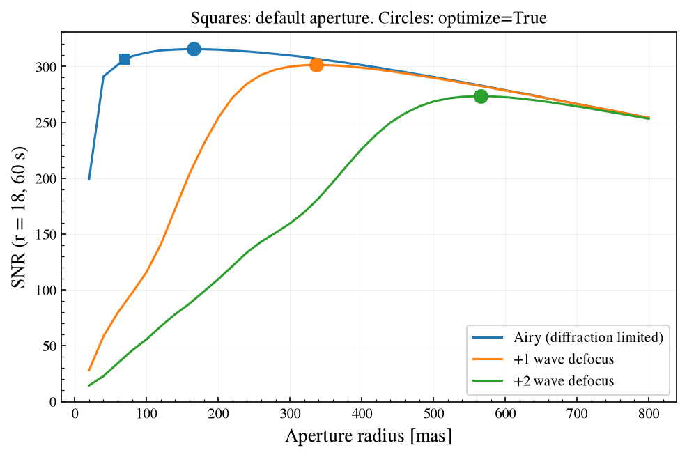
get_image_snr(time, psf=..., r_aper_mas=...) computes the SNR inside a fixed aperture, and optimize=True searches for the radius that maximizes it. plot_snr_vs_aperture draws the curve and marks two points on it: a square at the aperture get_image_snr uses by default, a circle at the optimum.

For the Airy PSF the default 70 mas aperture is already close to the optimum. For the defocused PSFs the default aperture follows the PSF instead, so the square and the circle coincide there; a 70 mas aperture on a two-wave PSF would hold only a few percent of the light.

radii = np.linspace(20, 800, 40)

fig, ax = plt.subplots(figsize=(7.6, 4.6))
for name, psf in PSFS.items():
    sim.plot_snr_vs_aperture(radii, time=60, psf=psf, ax=ax, label=name)
    default = sim.get_image_snr(time=60, psf=psf)
    best = sim.get_image_snr(time=60, psf=psf, optimize=True)
    print(
        f"{name:<28}"
        f" default r={default['r_aper_mas']:6.1f} mas SNR={default['snr']:7.2f}"
        f"   optimized r={best['r_aper_mas']:6.1f} mas SNR={best['snr']:7.2f}"
    )

ax.set_ylabel("SNR (r = 18, 60 s)")
ax.set_title("Squares: default aperture. Circles: optimize=True")
plt.show()

Airy (diffraction limited)   default r=  69.6 mas SNR= 306.74   optimized r= 166.1 mas SNR= 315.69
+1 wave defocus              default r= 336.4 mas SNR= 301.46   optimized r= 336.4 mas SNR= 301.46
+2 wave defocus              default r= 566.2 mas SNR= 273.47   optimized r= 566.2 mas SNR= 273.47

5. Bokeh backend

The image, radial and encircled-energy plots have a bokeh variant via backend='bokeh'. In a notebook call output_notebook() once and show(...) the returned figure; for the web portal pass return_='components' (script + div) or return_='html' instead.

from bokeh.io import output_notebook, show

output_notebook()
show(res.plot_image(backend="bokeh", units="mas", title="Airy PSF (bokeh)"))

Loading BokehJS ...

Summary

• AiryPSF, DefocusPSF and CustomPSF render normalized PSFs onto the detector grid, aware of pixel size and jitter.

• ImageSimulator.render_psf(psf, jitter_sigma_mas=..., npix=...) returns that bare PSF and plot_psf draws it; plate_scale_mas converts pixels to mas for the radial and encircled-energy helpers.

• simulate(time) returns a SimulatedImage that plots itself.

• get_image_snr(time, psf=..., r_aper_mas=... | optimize=True) is the PSF-aware SNR, and plot_snr_vs_aperture shows how the aperture choice matters.