Note

This page is generated from the Jupyter notebook notebooks/06_source_spectra.ipynb in the repository. You can download it and run it interactively.

Parametric source spectra

Besides Pickles spectral types and on-disk spectra, get_scene(name=...) builds a source spectrum on the fly from four parametric types:

name	params	meaning
blackbody	teff (K)	Planck spectrum, normalized to mag
flat	flat_unit ('fnu' or 'flam')	constant in F_nu (AB flat, default) or in F_lambda
powerlaw	alpha	F_lambda proportional to (lambda / lambda_ref) ** alpha
emission	lines=[{wave, flux, fwhm}], mag=None	sum of Gaussian lines with absolute fluxes

Each is a normal scene source, so the SNR machinery and update work as for any other spectrum. Every source element draws itself with .plot(ax=...).

import matplotlib.pyplot as plt
import numpy as np

import wcc_etc

wcc_etc.set_wcc_style()

BKG = {"bandpass": "johnson_r", "mag": 22.5}
WAVE = np.arange(3500, 9500, 5.0)  # optical plotting grid [Angstrom]


def source(name, **kw):
    """The source element of a scene of the given type, on a zodi background."""
    kw.setdefault("bandpass", "johnson_r")
    return wcc_etc.get_scene(
        name=name, background="zodi", background_prop=BKG, **kw
    ).source

1. Blackbody

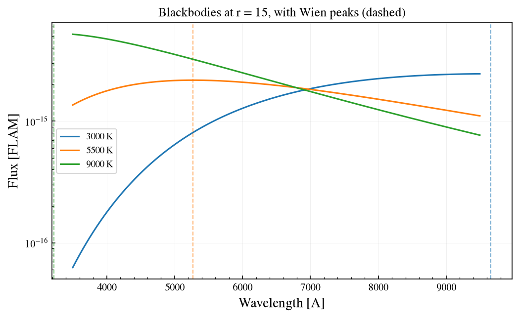
name='blackbody', teff=<K> builds a Planck spectrum normalized to the requested broadband magnitude. Dashed lines mark the Wien peak, lambda_max = 2.898e7 / T Angstrom.

fig, ax = plt.subplots(figsize=(8, 4.5))
for teff in (3000, 5500, 9000):
    src = source("blackbody", teff=teff, mag=15)
    src.plot(ax=ax, wave=WAVE, flux_unit="flam", label=f"{teff} K")
    ax.axvline(
        2.8977719e7 / teff, color=ax.lines[-1].get_color(), ls="--", lw=1, alpha=0.6
    )

ax.set_yscale("log")
ax.set_title("Blackbodies at r = 15, with Wien peaks (dashed)")
ax.legend(fontsize=9)
plt.show()

2. Flat

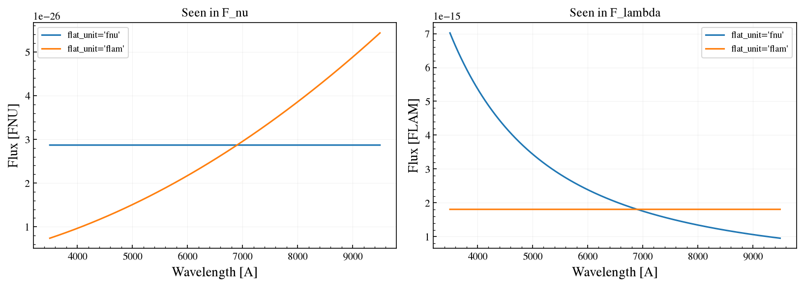
name='flat' defaults to flat_unit='fnu', flat in F_nu, which is the AB reference and falls as lambda squared in F_lambda. flat_unit='flam' is flat in F_lambda instead.

fig, (ax_fnu, ax_flam) = plt.subplots(1, 2, figsize=(11, 4))
for unit in ("fnu", "flam"):
    src = source("flat", flat_unit=unit, mag=15)
    src.plot(ax=ax_fnu, wave=WAVE, flux_unit="fnu", label=f"flat_unit='{unit}'")
    src.plot(ax=ax_flam, wave=WAVE, flux_unit="flam", label=f"flat_unit='{unit}'")

ax_fnu.set_title("Seen in F_nu")
ax_flam.set_title("Seen in F_lambda")
for ax in (ax_fnu, ax_flam):
    ax.legend(fontsize=9)
fig.tight_layout()
plt.show()

3. Power law

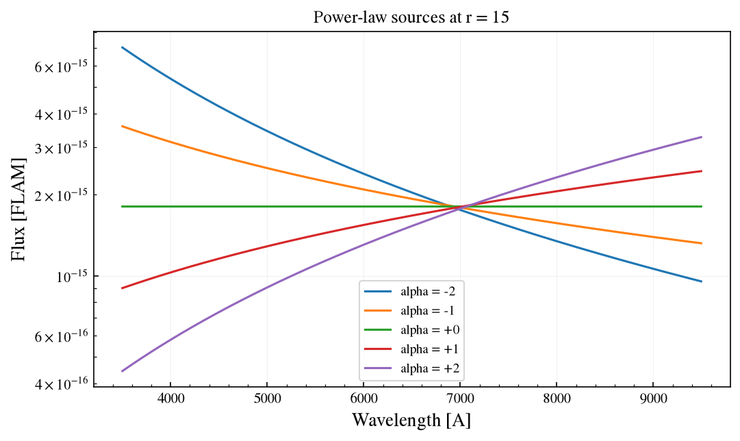
name='powerlaw', alpha=<exponent> builds F_lambda proportional to (lambda / lambda_ref) ** alpha. The public alpha is the F_lambda exponent, so alpha=0 is flat in F_lambda, negative is red, positive is blue.

fig, ax = plt.subplots(figsize=(8, 4.5))
for alpha in (-2.0, -1.0, 0.0, 1.0, 2.0):
    source("powerlaw", alpha=alpha, mag=15).plot(
        ax=ax, wave=WAVE, flux_unit="flam", label=f"alpha = {alpha:+.0f}"
    )

ax.set_yscale("log")
ax.set_title("Power-law sources at r = 15")
ax.legend(fontsize=9)
plt.show()

4. Emission lines

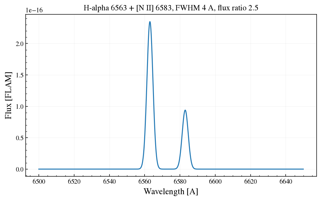
name='emission', mag=None, lines=[{wave, flux, fwhm}] sums Gaussian profiles. flux is the absolute integrated line flux in erg/s/cm^2 and fwhm defaults to 2 Angstrom. With mag=None the source carries absolute flux and is not broadband-normalized. Passing a magnitude together with absolute line fluxes raises, since the two would disagree about the flux scale.

src = source(
    "emission",
    mag=None,
    lines=[
        {"wave": 6563, "flux": 1e-15, "fwhm": 4},  # H-alpha
        {"wave": 6583, "flux": 4e-16, "fwhm": 4},  # [N II]
    ],
)

fig, ax = plt.subplots(figsize=(8, 4.5))
src.plot(ax=ax, wave=np.arange(6500, 6650, 0.05), flux_unit="flam")
ax.set_title("H-alpha 6563 + [N II] 6583, FWHM 4 A, flux ratio 2.5")
plt.show()

5. Driving the ETC

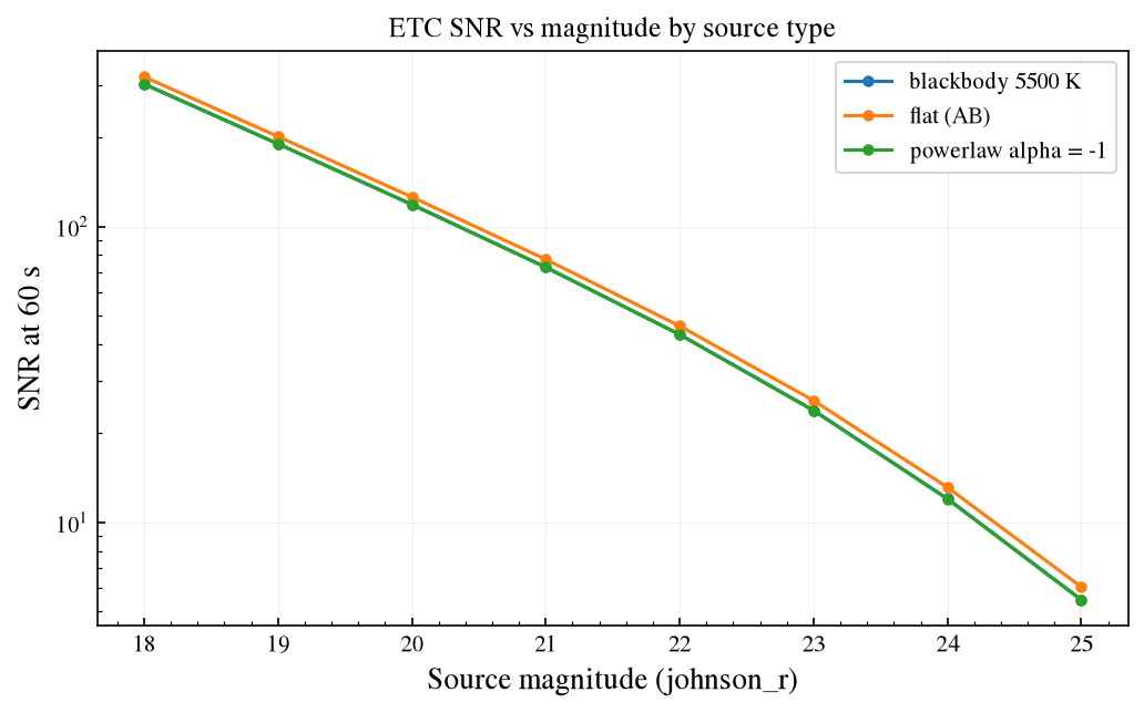
Each continuum source feeds the full Simulation through the broadband sony:r filter. plot_snr_vs_mag sweeps the source magnitude off a single cached render, so one simulation per source type is enough. The SNR follows Pogson scaling: five magnitudes fainter is a hundredth of the count rate.

Emission-line sources can also be observed through the H-alpha filters zwo:halpha2, zwo:halpha6 and zwo:halpha20 (2, 6 and 20 nm wide) with from_sensorfilter. zwo:hbeta and zwo:heii are placeholders without a throughput curve yet.

SPECS = {
    "blackbody 5500 K": ("blackbody", {"teff": 5500}),
    "flat (AB)": ("flat", {}),
    "powerlaw alpha = -1": ("powerlaw", {"alpha": -1.0}),
}
mags = np.linspace(18, 25, 8)

fig, ax = plt.subplots(figsize=(8, 4.5))
for label, (name, extra) in SPECS.items():
    scene = wcc_etc.get_scene(
        name=name,
        mag=18,
        background="zodi",
        bandpass="johnson_r",
        background_prop=BKG,
        **extra,
    )
    sim = wcc_etc.Simulation.from_sensor_and_scene("sony:r", scene)
    sim.plot_snr_vs_mag(mags, time=60, ax=ax, marker="o", ms=4, label=label)

ax.set_yscale("log")
ax.set_xlabel("Source magnitude (johnson_r)")
ax.set_ylabel("SNR at 60 s")
ax.set_title("ETC SNR vs magnitude by source type")
plt.show()

[wcc_etc] note: even n_pixels is rounded up by 1 to center the PSF peak (shown once).

6. update() rebuilds the spectrum

Shape parameters of a parametric source change in place and rebuild the spectrum. The spectrum type is locked: there is no source__spectrum key, so sim.update(source__spectrum=...) raises KeyError. Build a new scene to change the type.

At a fixed r = 19 normalization, dropping the blackbody from 8000 K to 3000 K changes the SED under the broad r filter and with it the count rate.

scene = wcc_etc.get_scene(
    name="blackbody",
    teff=8000,
    mag=19,
    background="zodi",
    bandpass="johnson_r",
    background_prop=BKG,
)
sim = wcc_etc.Simulation.from_sensor_and_scene("sony:r", scene)

print(f"SNR at teff = 8000 K : {sim.get_snr(60)['snr']:.1f}")
sim.update(
    source__teff=3000
)  # cooler blackbody, less r-band flux per unit of normalization
print(f"SNR at teff = 3000 K : {sim.get_snr(60)['snr']:.1f}")

try:
    sim.update(source__spectrum="powerlaw")
except KeyError as err:
    print("update(source__spectrum=...) ->", err)

SNR at teff = 8000 K : 202.4
SNR at teff = 3000 K : 155.7
update(source__spectrum=...) -> "no entries found matching key='source__spectrum'"

7. Normalization bandpass

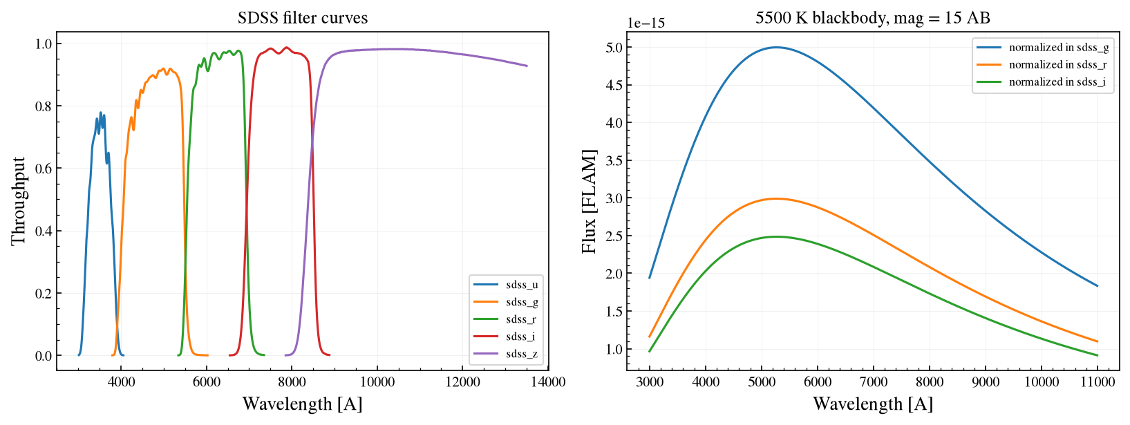
bandpass sets the filter the source magnitude is anchored in. Alongside synphot’s built-in systems the ETC ships the SDSS filters as local curves: sdss_u, sdss_g, sdss_r, sdss_i, sdss_z, accepted anywhere a bandpass name is. SDSS magnitudes are AB, so pass magsys="abmag" with them. plot_bandpass_mpl draws any bandpass.

from wcc_etc.io import resolve_bandpass

fig, (ax_bp, ax_norm) = plt.subplots(1, 2, figsize=(11, 4.2))

for name in ["sdss_u", "sdss_g", "sdss_r", "sdss_i", "sdss_z"]:
    wcc_etc.plot_bandpass_mpl(resolve_bandpass(name), ax=ax_bp, label=name)
ax_bp.set_title("SDSS filter curves")
ax_bp.legend(fontsize=8)

for name in ["sdss_g", "sdss_r", "sdss_i"]:
    source("blackbody", teff=5500, mag=15, magsys="abmag", bandpass=name).plot(
        ax=ax_norm,
        wave=np.arange(3000, 11000, 5.0),
        flux_unit="flam",
        label=f"normalized in {name}",
    )
ax_norm.set_title("5500 K blackbody, mag = 15 AB")
ax_norm.legend(fontsize=8)

fig.tight_layout()
plt.show()

Summary

• blackbody: Planck spectrum normalized to mag; the peak follows Wien’s law.

• flat: AB flat (fnu) falls as lambda squared in F_lambda; flam is constant in F_lambda.

• powerlaw: F_lambda follows (lambda / lambda_ref) ** alpha, with alpha the F_lambda exponent.

• emission: Gaussian lines with absolute fluxes; use mag=None.

• plot_snr_vs_mag sweeps the magnitude of any of them off one render.

• update rebuilds the shape parameters in place; the spectrum type is fixed.

• bandpass picks the normalization filter; the SDSS curves ship with the package.