Note

This page is generated from the Jupyter notebook notebooks/03_from_sensorfilter.ipynb in the repository. You can download it and run it interactively.

from_sensorfilter: the PSF follows the filter

Simulation.from_sensorfilter and ImageSimulator.from_sensorfilter build from a canonical sensorfilter label (kind:band, e.g. 'zwo:r'). Compared with from_sensor_and_scene they do two extra things:

1. pick the throughput curve for that filter position, and

2. pick the PSF that matches the filter’s focus level, so defocused filters get a defocused PSF without a psf= argument.

The chosen PSF is exposed as default_psf and used by get_snr, simulate, render_psf, get_peak_pixel and get_image_exptime_for_snr whenever psf= is omitted.

import matplotlib.pyplot as plt
import numpy as np

import wcc_etc

wcc_etc.set_wcc_style()

scene = wcc_etc.get_scene(
    name="G5V",
    mag=19,
    background="zodi",
    bandpass="johnson_r",
    background_prop={"bandpass": "johnson_r", "mag": 22.5},
)

LABELS = ["zwo:r", "zwo:r+1", "zwo:bb2"]

1. Label to PSF

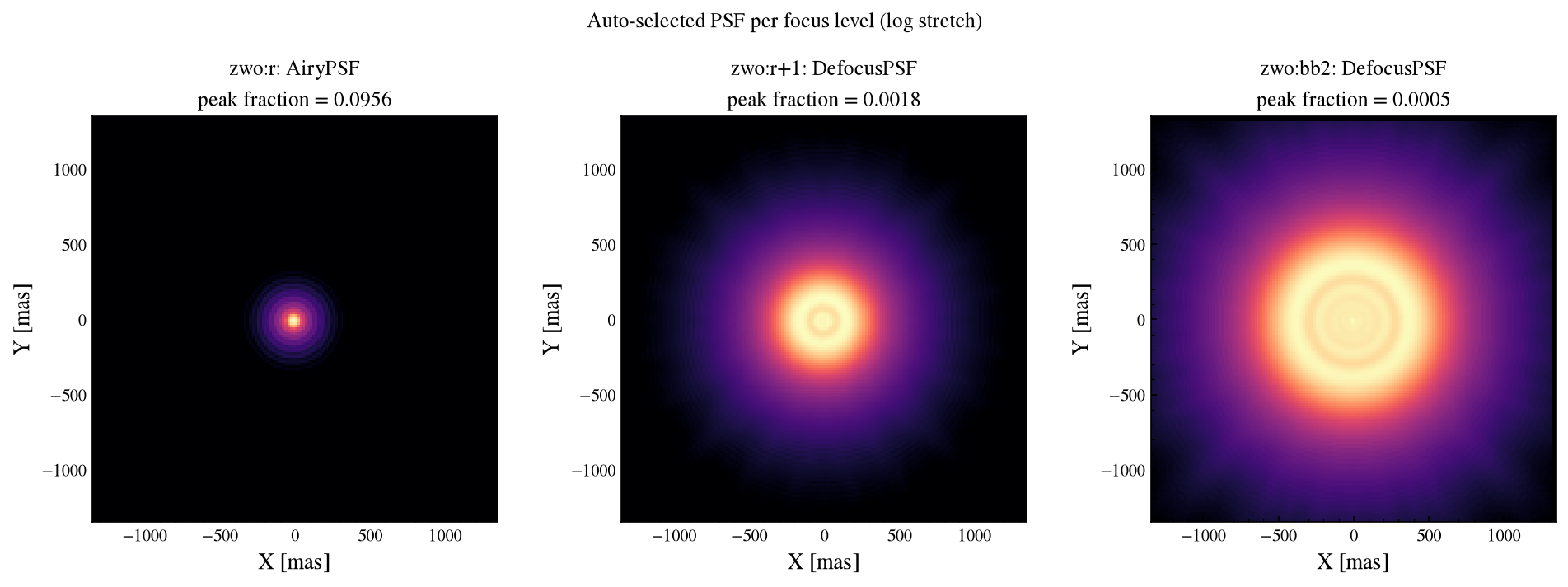
The suffix on the band names the focus level: no suffix is in focus, +1 and -1 are one wave either side of focus, and 2 is two waves out. zwo:r, zwo:r+1, zwo:r-1 and zwo:bb2 are the labels in the current layout. default_psf reports what was selected.

for label in LABELS:
    sim = wcc_etc.Simulation.from_sensorfilter(label, scene)
    print(f"{label:<10}{type(sim.default_psf).__name__}")

zwo:r     AiryPSF
zwo:r+1   DefocusPSF
zwo:bb2   DefocusPSF

2. What the auto-selected PSFs look like

ImageSimulator.plot_psf() renders the filter’s own PSF on the detector grid, normalized to unit sum and on a log stretch. The in-focus image is a tight Airy core; the one- and two-wave images spread the light into progressively larger rings. Each title also quotes the peak-pixel fraction, which is what the saturation budget in notebook 02 depends on.

fig, axes = plt.subplots(1, 3, figsize=(13, 4.4))
for ax, label in zip(axes, LABELS):
    imsim = wcc_etc.ImageSimulator.from_sensorfilter(
        label, scene, npix=160, oversample=5
    )
    peak = imsim.render_psf().max()
    imsim.plot_psf(
        ax=ax,
        cmap="magma",
        colorbar=False,
        title=f"{label}: {type(imsim.default_psf).__name__}\n"
        f"peak fraction = {peak:.4f}",
    )

fig.suptitle("Auto-selected PSF per focus level (log stretch)", y=1.02)
fig.tight_layout()
plt.show()

[wcc_etc] note: even n_pixels is rounded up by 1 to center the PSF peak (shown once).

3. Defocus and filter width

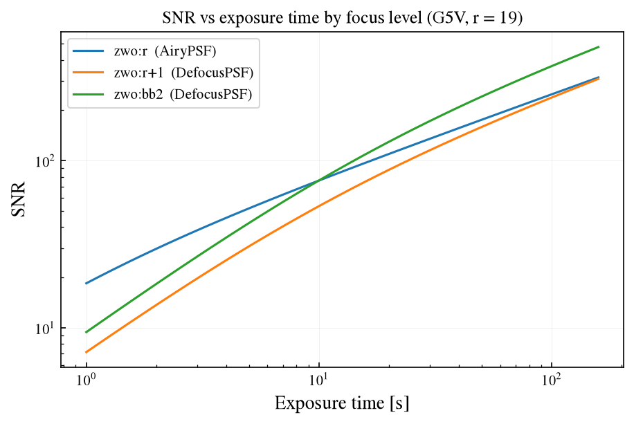
Spreading the same photons over more pixels means more noise pixels inside the aperture. zwo:r+1 is the r filter one wave out of focus, so comparing it with zwo:r isolates that cost; the aperture follows the PSF in both cases. zwo:bb2 is a different filter, the broad band two waves out of focus, and it collects enough extra photons to land above the in-focus r band in spite of the blur. At 60 s on this r = 19 star one wave of defocus costs about 8 percent in SNR. plot_snr takes the array of times directly and draws one curve per simulation; no psf= is passed anywhere.

times = np.logspace(0, 2.2, 40)

fig, ax = plt.subplots(figsize=(7, 4.2))
for label in LABELS:
    sim = wcc_etc.Simulation.from_sensorfilter(label, scene)
    sim.plot_snr(times, ax=ax, label=f"{label}  ({type(sim.default_psf).__name__})")
    at60 = sim.get_snr(60)
    print(
        f"{label:<10} SNR at 60 s = {at60['snr']:6.1f}   "
        f"aperture {at60['r_aper_mas']:5.1f} mas"
    )

ax.set_xscale("log")
ax.set_yscale("log")
ax.set_title("SNR vs exposure time by focus level (G5V, r = 19)")
plt.show()

zwo:r      SNR at 60 s =  192.7   aperture  69.6 mas
zwo:r+1    SNR at 60 s =  177.5   aperture 300.9 mas
zwo:bb2    SNR at 60 s =  271.0   aperture 560.0 mas

4. Guards

from_sensorfilter accepts only canonical labels that have a throughput curve. An unknown label raises ValueError; a known filter with no curve yet (the narrowband placeholders) raises NotImplementedError. Nicknames such as 'sony:r' are not canonical here. Use from_sensor_and_scene for those, or 'zwo:r'.

for label in ["zwo:does_not_exist", "zwo:hbeta", "sony:r"]:
    try:
        wcc_etc.Simulation.from_sensorfilter(label, scene)
    except (ValueError, NotImplementedError) as err:
        print(f"{label:<20}{type(err).__name__}: {str(err)[:70]}...")

zwo:does_not_exist  ValueError: Unknown sensorfilter 'zwo:does_not_exist'. Known labels: ['qcmos:bb', ...
zwo:hbeta           NotImplementedError: Sensorfilter 'zwo:hbeta' is not yet implemented (no throughput curve a...
sony:r              ValueError: Unknown sensorfilter 'sony:r'. Known labels: ['qcmos:bb', 'qcmos:g', '...

Summary

• Simulation.from_sensorfilter(label, scene) and ImageSimulator.from_sensorfilter(label, scene, npix=..., oversample=...) build from a canonical kind:band label.

• The PSF comes from the filter’s focus level and is exposed as default_psf (AiryPSF in focus, DefocusPSF for the +1 and 2 suffixes).

• imsim.plot_psf() shows it; sim.plot_snr(times) shows what the defocus costs.

• Unknown labels raise ValueError, unimplemented ones NotImplementedError.