Signal-to-noise and exposure time
wcc-etc has two SNR paths, which agree to about 1% for an in-focus point
source, and the exposure-time inverse of each. The image-based path is the
default; the analytic Airy path is kept for cross-checks.
What goes into the SNR
The image-based path renders the PSF on the detector grid, scales it to the source count rate, adds the host, the sky and the dark current, and then does circular-aperture photometry on that frame. For an aperture of \(n_{pix}\) pixels and an exposure of \(t\) seconds the result is the usual CCD equation,
where \(S\) is the source charge inside the aperture (the total source
charge times the enclosed fraction of the PSF), \(H\) the charge from an
unresolved host that rides the same PSF, \(B\) the sky rate per pixel,
\(D\) the dark rate per pixel, \(E\) the per-pixel rate of any
resolved element such as a Sersic host, and \(\sigma_R\) the read noise
per read. Only \(S\) is signal. Everything else contributes shot noise and
fills the well, and that is what the host slot in a scene is for (see
Scenes, sources, and backgrounds).
The balance of these terms decides how the SNR scales. When the source dominates, SNR grows as the square root of the exposure time and gains a factor of about 1.6 per magnitude. When sky or read noise dominates, SNR grows linearly with the source and a magnitude costs a factor of 2.5. The two sensors below cross from one regime to the other at different magnitudes because the qCMOS has far lower read noise:
import numpy as np
import matplotlib.pyplot as plt
import wcc_etc
from wcc_etc import get_scene, Simulation

wcc_etc.set_wcc_style()

scene = get_scene("G5V", mag=20, background="zodi", bandpass="johnson_r")

fig, (ax_mag, ax_t) = plt.subplots(1, 2, figsize=(11, 4))
for label in ("sony:r", "qcmos:r"):
    sim = Simulation.from_sensor_and_scene(label, scene)
    sim.plot_snr_vs_mag(np.arange(14, 25), time=60, ax=ax_mag, label=label)
    sim.plot_exptime_for_snr([5, 10, 20, 50, 100], ax=ax_t, label=label)
ax_mag.set_yscale("log")
ax_t.set_yscale("log")
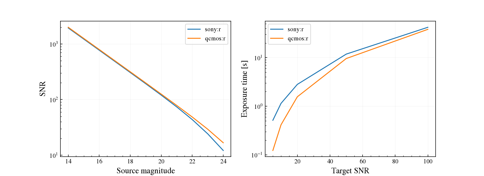
Image-based SNR (the default)
get_snr() delegates to
get_image_snr() and returns a dictionary:
r = sim.get_snr(time=60)
r["snr"]                 # signal-to-noise ratio
r["signal_e"]            # source electrons inside the aperture
r["noise_e"]             # total noise (electrons)
r["enclosed_fraction"]   # PSF fraction inside the aperture
r["r_aper_mas"]          # aperture radius (mas)
r["n_pix"]               # number of pixels in the aperture
r["n_saturated"]         # pixels at/above full well in the per-frame image
r["saturated"]           # bool
Important
The return value is a dict, so index ["snr"]. Earlier versions returned
a Quantity with .value.
Choosing the aperture
Aperture precedence is optimize, then r_aper_mas, then ee_frac.
If none is given, the aperture follows the PSF: 70 mas for the in-focus Airy
PSF, the SNR-optimized radius for a defocused filter (zwo:r+1,
zwo:bb2, …), or the Simulation’s own r_aper_mas if one was set at
construction.
sim.get_snr(60, r_aper_mas=300)          # fixed aperture radius (mas)
sim.get_snr(60, ee_frac=0.8)             # aperture enclosing 80% of the PSF
sim.get_snr(60, optimize=True)           # radius that maximizes SNR
plot_snr_vs_aperture() draws SNR against aperture
radius and marks the default and the optimized choice, which is the quickest
way to see how much a wrong aperture costs.
Sweeping time or magnitude
time may be a scalar or an array. get_image_snr also accepts
mags to sweep the source brightness off a single cached render, with the
host, background, dark and read noise held fixed. time and mags may
not both be arrays.
import numpy as np
sim.get_snr(time=np.array([10, 30, 60, 120]))["snr"]      # array of SNR
sim.get_image_snr(time=60, mags=np.arange(16, 24))["snr"] # SNR vs. magnitude
The same sweeps as plots are plot_snr() (SNR
against time, also reachable as sim.plot) and
plot_snr_vs_mag().
Specifying the PSF and jitter
Pass any PSFSource, and override the jitter per
call:
from wcc_etc import DefocusPSF, DEFOCUS_2WAVE_PATH
sim.get_image_snr(time=60, psf=DefocusPSF(DEFOCUS_2WAVE_PATH))
sim.get_image_snr(time=60, jitter_sigma_mas=15)
See PSFs and image simulation for the PSF models and the npix / oversample grid
parameters.
Exposure time for a target SNR
get_image_exptime_for_snr() inverts the image-based
SNR. get_exptime_for_snr() is the analytic Airy
inverse that pairs with get_snr_airy.
sim.get_image_exptime_for_snr(snr=100)        # seconds (PSF-aware)
sim.get_exptime_for_snr(snr=100)              # seconds (analytic Airy)
plot_exptime_for_snr() draws the first of these for
a list of target SNRs, as in the right-hand panel above.
Multiple reads (n_reads)
Splitting an exposure into several reads adds read noise once per read, so
the read term in the SNR grows with n_reads. All SNR and exposure-time
methods accept n_reads, and the default comes from the sensor or the
simulation’s meta:
sim.get_snr(60, n_reads=4)
sim.get_image_exptime_for_snr(snr=100, n_reads=4)
The reason to pay that price is saturation, which is tested per frame (see
Saturation). sim.plot_sweep("n_reads", [1, 2, 4, 8], time=60)
shows the cost for a given exposure.
The analytic Airy SNR
get_snr_airy() is the original closed-form
Airy-disk approximation. It is kept for cross-checking the image-based path
and emits a DeprecationWarning. To use it quietly:
import warnings
with warnings.catch_warnings():
    warnings.simplefilter("ignore", DeprecationWarning)
    snr_airy = sim.get_snr_airy(60)
For an in-focus AiryPSF with the default aperture, the
image-based and analytic results agree to about 1%. The analytic path cannot
place a Sersic host and warns that it ignores one.